Examining State-to-State Geographic Mobility

.. tools, resources and insights to examine U.S. by state migration 2011-2017 and migration flows in 2016 .. this post is an excerpt from the more detailed Web page http://proximityone.com/statemigration.htm.

In examining future demographic trends, the most challenging component of change to project (develop data values into the future) is migration. Migration, comprised net domestic and net international migration, is a function of many factors whose cause and effect behavior can change year by year, and geographic area by area. While this section is focused on states, the same scope of data is available to the county and sub-county levels. In this section, U.S. by state migration is examined using two data sources: annual population and components of change model-based estimates (2010-2017 model-based estimates) and annual American Community Survey estimates (ACS 2016 estimates). While these Census Bureau programs are highly related, the migration data/subject matter differ some.

State Net Domestic Migration, 2011-2017
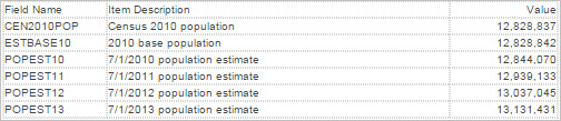
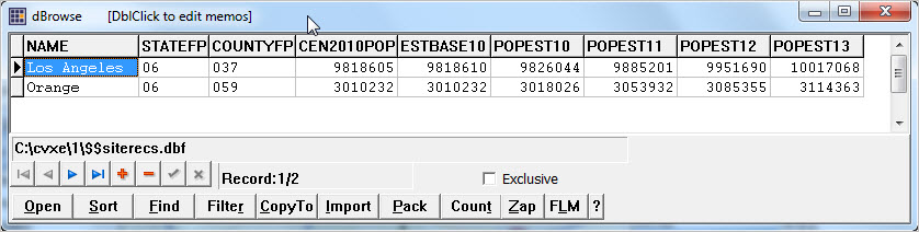
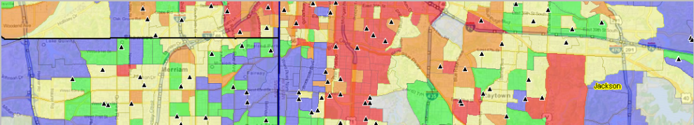
The following graphic shows patterns net domestic migration for the period 2011-2017, based on the model-based estimates. The patterns of migration change, direction and magnitude are immediately evident. Click on the graphic to see a larger view showing more detail. Expand browser to full screen for best quality view. The larger view shows a portion of a mini-profile for Florida. The mini-profile illustrates how these data are comprised … annual net domestic migration estimates and the sum over the years 2011-2017. See the interactive table to view these data, and related components of change, in a tabular, numeric form. Use the GIS project (details here) to create similar views for any state; visual analysis of outmigration for any state showing outmigration by destination state. Label areas as desired. Add other layers. Add your own data.

View created with CV XE GIS. Click graphic for larger view with more detail.

State OutMigration by Destination State
The model-based estimates, reviewed above, do not provide detail on state-to-state migration. Those data are provided by the related ACS 2016 estimates. Note that the ACS 2016 1-year estimates are for the calendar year 2016. From these data we can get the following migration detail … In 2016, there were an estimated 605,018 people who moved from a residence 1 year earlier, in a different state, to Florida. Florida experienced the largest number of movers (inflows) from other states among all states. 60,472 of these movers were from New York. See the interactive table in this section to examine similar characteristics for any state. These data are based on the 2016 ACS 1 year estimates. See about related data.

The American Community Survey (ACS) asks respondents age 1 year and over whether they lived in the same residence 1 year ago. For people who lived in a different residence, the location of their previous residence is collected. The state-to-state migration flows are created from tabulations of the current state (including the District of Columbia) of residence crossed by state of residence 1 year ago.

Movers Within and Between States & Selected Areas During 2016
Use the interactive table to examine state outmigration by destination state. View, compare, query, rank and export data of interest.

Data Analytics Web Sessions
.. is my area urban, rural or …
.. how do census blocks relate to congressional district? redistricting?
.. how can I map census block demographics?
Join me in a Data Analytics Web Session, every Tuesday, where we review access to and use of data, tools and methods relating to GeoStatistical Data Analytics Learning. We review current topical issues and data — and how you can access/use tools/data to meet your needs/interests.

About the Author
Warren Glimpse is former senior Census Bureau statistician responsible for innovative data access and use operations. He is also the former associate director of the U.S. Office of Federal Statistical Policy and Standards for data access and use. He has more than 20 years of experience in the private sector developing data resources and tools for integration and analysis of geographic, demographic, economic and business data. Contact Warren. Join Warren on LinkedIn.

Census Block, Block Group & Census Tract GeoDemographics

Census tracts, block groups and blocks are the important small area statistical geographic areas for which data from Census 2010 are tabulated. Data for census tracts and block groups are also tabulated annually from the American Community Survey. For example. in December 2018, we will have new “richer demographics” annual estimates centric to each year 2008 through 2015 for Census 2010 tracts and block groups … data such as educational attainment, language spoken, housing and household characteristics,  income characteristics and employment and other demographic-economic attributes.

Largest Population New York City (NYC) Census Blocks
The following graphic shows the NYC Census 2010 census block having the largest Census 2010 population that is not a group quarters population block. The Lincoln Center census block shown in the graphic (red boundary) has 4,067 population and 2,922 housing units.

– click graphic for larger view; view developed using CV XE GIS

This block (36 061 015500 6000) occupies 0.033 square miles. It has a population density of 122,333 (population per square mile). The NYC block with the largest population is on Rikers Island and has a group quarters population of 8,634 and 0 housing units. For Census 2010, there were 350,169 census blocks covering the state of New York; 13,356 census blocks were water blocks. For the State of New York, as of Census 2010 the average census block population was 55 (57 excluding water blocks).

Census 2010 and Census 2020
These geographies have generally stable geographic areas and codes from one decennial census (e.g., Census 2010) to the next (e.g., Census 2020). Many of these areas will change in terms of code and area for Census 2020, though the geographic changes will typically be small or not at all.

Census 2020 block, block group and tract codes and geometry will be available in late 2020. Initial block level demographics will be available in March 2021.

Census 2010 & Current GeoDemographics
These areas cover the U.S. from wall-to-wall and generally non-changing in terms of boundary and geographic code (geocode) until Census 2020. This section provides a summary of new Web pages with more detail about each of these geographies:
• census tracts and tract codes .. 73,056 areas
• census block groups and block group codes .. 217,740 areas
• census blocks and block codes .. 11,078,297 areas

Each of these pages provides an interactive table to view tallies of Census 2010 for each of these small area geographies.

Combining Address Data with Small Area Geography
The address of the Office of the California Secretary of State, located at 1500 11th St, Sacramento, CA 95814, was geocoded using the APIGeocoder and converted into a shapefile for Geographic Information System applications.  The location is shown as a red marker in the map views shown below, illustrating each type of small area geography: tracts. block groups and blocks.

Census Tracts
Tracts are labeled with green tract codes. Address 1500 11th St, Sacramento, CA 95814 is shown by red marker.  The address is in tract 06067001101.

View created using CV XE GIS.

Block Groups
Block groups are labeled with red block group codes.  Tract 06067001101 is comprised of block groups: 060670011011 and 060670011012.  See pointer in map view; the block group within tract boundary.

View created using CV XE GIS.

Zoom-in to Census Block
Blocks are labeled with yellow block codes. The address is located in block 060670011011085.

View created using CV XE GIS.

Further Zoom-in Showing Streets
Streets are labeled with street names. Identify tool is used to show mini-profile for 1500 block of 11th Street.

View created using CV XE GIS.

Is the tract code 11.01 or 001101?
Both. Census tracts within a county are identified by a 4-digit basic code between 0001 and 9999, and may have a 2-digit suffix ranging from .01 to .98; for example, 6059.02. The decimal point separating the 4-digit basic tract code from the 2-digit suffix is shown in Census Bureau printed reports and maps. For geo-referencing, the decimal point is implied and does not appear; the 6-character tract code with lead zeroes is used — a character string with no blanks and all numbers.

Accessing and Using these Geographies & Related Demographics
There are several ways these geographies can be used.
• The geocodes are the “handles” to access demographic-economic statistical data.
• The geographies may be visually, geospatially, related as shapefiles.
.. the Census Bureau makes these shapefiles available for use in user appications.
.. the shapefiles typically do not include demographic-economic data.

Access Census 2010 Census Block (and Block Group/Tract) data:
• P.L. 94-171 Redistricting Data — http://proximityone.com/cen2010_pl94171.htm
• Summary File 1 — http://proximityone.com/cen2010_sf1.htm

Access Census Block Group and Tract richer demographics:
• 2016 American Community Survey (ACS) 5-year estimates
  — http://proximityone.com/acs1216.htm
• Access annual counterparts to above section
• Census blocks — http://proximityone.com/cenblk.htm
• Census block groups — http://proximityone.com/blockgroups.htm
• Census tracts — http://proximityone.com/tracts.htm

Alternatively use the Census Bureau APIs or CV XE GIS APIGateway.

Data Analytics Web Sessions
.. is my area urban, rural or …
.. how do census blocks relate to congressional district? redistricting?
.. how can I map census block demographics?
Join me in a Data Analytics Web Session, every Tuesday, where we review access to and use of data, tools and methods relating to GeoStatistical Data Analytics Learning. We review current topical issues and data — and how you can access/use tools/data to meet your needs/interests.

About the Author
Warren Glimpse is former senior Census Bureau statistician responsible for innovative data access and use operations. He is also the former associate director of the U.S. Office of Federal Statistical Policy and Standards for data access and use. He has more than 20 years of experience in the private sector developing data resources and tools for integration and analysis of geographic, demographic, economic and business data. Contact Warren. Join Warren on LinkedIn.

State and Regional Decision-Making Information

Organized on a state-by-state basis, use tools and geographic, demographic and economic data resources in these sections to facilitate planning and analysis. Updated frequently, these sections provide a unique means to access to multi-sourced data to develop insights into patterns, characteristics and trends on wide-ranging issues. Bookmark the related main Web page; keep up-to-date.

Using these Resources
Knowing “where we are” and “how things have changed” are key factors in knowing about the where, when and how of future change — and how that change might impact you. There are many sources of this knowledge. Often the required data do not knit together in an ideal manner. Key data are available for different types of geography, become available at different points in time and are often not the perfect subject matter. These sections provide access to relevant data and a means to consume the data more effectively than might otherwise be possible. Use these data, tools and resources in combination with other data to perform wide-ranging data analytics. See examples.

Select a State/Area

Alabama Alaska Arizona Arkansas California Colorado Connecticut Delaware D.C. Florida Georgia Hawaii Idaho Illinois Indiana Iowa Kansas

Kentucky Louisiana Maine Maryland Massachusetts Michigan Minnesota Mississippi Missouri Montana Nebraska Nevada New Hampshire New Jersey New Mexico New York North Carolina

North Dakota Ohio Oklahoma Oregon Pennsylvania Rhode Island South Carolina South Dakota Tennessee Texas Utah Vermont Virginia Washington West Virginia Wisconsin Wyoming

Topics for each State — with drill-down to census block
• Visual pattern analysis tools … using GIS resources
• Digital Map Database
• Situation & Outlook
• Metropolitan Areas
• Congressional Districts
• Counties
• Cities/Places
• Census Tracts
• ZIP Code Areas
• K-12 Education, Schools & School Districts
• Block Groups
• Census Blocks

Join me in a Data Analytics Lab session to discuss more details about accessing and using wide-ranging demographic-economic data and data analytics. Learn more about using these data for areas and applications of interest.

About the Author
— Warren Glimpse is former senior Census Bureau statistician responsible for innovative data access and use operations. He is also the former associate director of the U.S. Office of Federal Statistical Policy and Standards for data access and use. He has more than 20 years of experience in the private sector developing data resources and tools for integration and analysis of geographic, demographic, economic and business data. Contact Warren. Join Warren on LinkedIn.

Comparing Census Tract Demographics Over Time

.. it’s about more than census tracts .. this section is about comparing American Community Survey ACS 5-year estimates: 2005-2009 with 2010-2014 … something new and powerful happening this week.

To make good business decisions we need hard data, recent data, trend data … to assess patterns and change and develop reliable, superior plans. Read about the past and then how things have changed for the better.

Imagine that it is 2005. Data from Census 2000 are now 5 years old. There will not be another update for richer demographics for all counties and cities in the foreseeable further. There will not be any update for small area geography such as census tracts or block groups until Census 2010. Businesses are forced to use out-of-date data to assess markets … where and how are opportunities changing? City and neighborhood planners can only make educated guesses to respond to growing needs of various population groups. Federal and state government programs that base funding allocations on demographics are challenged. Changes in the rental vacancy rates for most cities, counties and metros will remain unknown for the foreseeable future.

Fast forward to 2015 and present day reality. The situation is now radically different. First, we can now compare 5-year estimates from the 2009 American Community Survey ACS to those from the 2014 ACS 5 year estimates. Second, we will be able to do that again in 2016 — compare 5-year estimates from ACS 2010 to those from ACS 2015. Health planners can now assess the size and change in special needs population and how that matches up to resources that respond to those needs — rather than guessing. Schools and school districts can better understand how school age population trending and plan for enrollment change. Education agencies are better able to assess how changing demographics among school systems compare to one-another. Businesses can now determine the size of potential markets and how they are trending based on hard data. It is possible to compare changing patterns in rental vacancy rates and rental housing market conditions for all levels of geography down to block group.

The American Community Survey ACS provides a wide range of important statistics about people and housing for every community in the nation. These data are the only source of local estimates for most of the approximately 40 topics it covers for even the smallest communities. It produces statistics for ancestry, language, education, commuting, employment, mortgage status and rent, as well as income, poverty and health insurance. The ACS estimates are tabulated annually as 1-year estimates (e.g., the ACS 2014 1-year estimates) and 5-year estimates (e.g., the ACS 2014 5-year estimates. See a comparison below in this section about scope, advantages/disadvantages, and other usage attributes for the 1-year versus 5-year estimates.

See ACS 2014 5-year main page for additional data access & use details.

Data from the 5-year estimates are available for all geographies down to the block group level regardless of population size. Starting with the ACS 2014 5-year estimates, for the first time, users will be able to compare two non-overlapping five-year periods 2005-09 and 2010-14. Looking ahead, data from the 2006-10 and 2011-15 (available December 2016) will be comparable … and so on. Over several years, a time-series of 5-year estimates, non-overlapping five-year periods, will evolve.

Comparing Geography Between 2005-09 & 2010-14 ACS 5-Year Data
The following graphic summarizes geographic tabulation areas for 2005-09 and 2010-14 ACS 5-year data. Use the corresponding Web table as a reference guide for comparing data over time. Links provided in the table enable you to navigate to selected data access tables. This Web-page table updates with new links; bookmark the page for re-visits.

Updates
Posts later this month will provide updates on this topics; new data and new data analytics tools. Join me in a Data Analytics Lab session to discuss use of these data using analytical tools and methods applied to your situation.

About the Author
— Warren Glimpse is former senior Census Bureau statistician responsible for innovative data access and use operations. He is also the former associate director of the U.S. Office of Federal Statistical Policy and Standards for data access and use. He has more than 20 years of experience in the private sector developing data resources and tools for integration and analysis of geographic, demographic, economic and business data. Contact Warren. Join Warren on LinkedIn.

Business Data Analytics: Methods & Tools

Business Data Analytics can help most any business more effectively reach goals and objectives. Whether a new or established business, serving a county or national market, similar tools and methods apply. See related Web version for more details.

• How can you examine patterns/characteristics of existing customers?
• Where are prospective customers and possible unknown opportunities?
• How do you best define your market area?
  – what geographies have the largest number of prospects?
• What are the sales potential in this market area?
  – what are the best measures to examine sales potential?
• What is your competitive position?
  – how many other establishments offer a similar service in your market area?
• How can your sales data identify geographic areas of opportunity?

Tools and methods described here can help answer these questions and facilitate strategic planning. Here are key steps to using Business Data Analytics in your business. These applications make use of a GIS project and data for a business located in the San Diego area. Click link to view graphics.
• Business locations
• Territories served
• Market characteristics
• Urban population by block; population by tract
• Customer locations
• Prospect locations
• Competitor locations
• Composite of above
• Related topics

Locations [goto top]
Where are the business locations/stores/operations
Blue triangle markers show existing locations. Are these the ideal locations?

— view created using CV XE GIS and associated Business Patterns GIS Project
— click graphic for larger showing details.

Territories Served [goto top]
What territories do locations serve? Are they developed correctly?
Territories for service/market areas are shown as color-shaded areas.
— flexibly re-define territories

— view created using CV XE GIS and associated Business Patterns GIS Project
— click graphic for larger showing details.

Market Characteristics [goto top]
What are the market characteristics?
Graphic shows patterns of median household income (MHI) by census tract;
— identifying areas with best opportunity
— examine wide-ranging demographic-economic characteristics
— market area tracts shown with cross-hatch pattern
— MHI intervsls/color correspondence shown in legend at left of map
— ranges can be customized/shifted to suit

— view created using CV XE GIS and associated Business Patterns GIS Project
— click graphic for larger showing details.

Urban Population by Block; Population by Tract [goto top]
Urban census blocks are shown with an orange fill pattern.
– examine scope of urban areas and how they relate to business development.
Census tract population is shown as a label for all tracts.
– identify population concentrations/attributes for small areas.

— view created using CV XE GIS and associated Business Patterns GIS Project
— click graphic for larger showing details.

Customers [goto top]
Red markers show existing customers.
— linked to customer/product database

— view created using CV XE GIS and associated Business Patterns GIS Project
— click graphic for larger showing details.

Prospects [goto top]
Orange and green markers show prospects based on different sources/criteria.

— view created using CV XE GIS and associated Business Patterns GIS Project
— click graphic for larger showing details.

Competitors [goto top]
What is the competitive position/where are competitors located?
Red triangle markers show where competitors are located.

— view created using CV XE GIS and associated Business Patterns GIS Project
— click graphic for larger showing details.

Composite View [goto top]
Integrating business operating environment.
Graphic shows zoom-in to Encinatas location with all features shown separately in above views.
Roads/streets have been added; optionally use for routing and locational analysis.

— view created using CV XE GIS and associated Business Patterns GIS Project
— click graphic for larger showing details.

Related Topics for Extended Analysis [goto top]
These extended topics make use of the data and analyses reviewed above. These topics will be covered in subsequent sections.

• Determining performance relative to the market characteristics
• Assessing impact of external and internal factors affecting operations
  – supply chain, labor force, costs, demand …
• Examining financial situation and outlook?
• Determining areas of missed opportunity
  – metros, hot spots within metros (tracts)
• Using collective data in models for predictive analyses
  – how might things change, when where and how?
• How to interpret statistical releases
  – determining which relevant, assessing implications for impact
• How to most effectively make team/collaborative/management decisions

About the Author
— Warren Glimpse is former senior Census Bureau statistician responsible for innovative data access and use operations. He is also the former associate director of the U.S. Office of Federal Statistical Policy and Standards for data access and use. He has more than 20 years of experience in the private sector developing data resources and tools for integration and analysis of geographic, demographic, economic and business data.

Mapping Block Group Data

.. demographic-economic patterns and characteristics can often be “masked” when using larger geographic areas such as counties and metros. Using data for small area geography such as census tracts and block groups can help identify clusters and areas of interest. Now, demographic-economic data for block groups (217,000 areas averaging 1,200 population covering the U.S. wall-to-wall) are tabulated annually from the American Community Survey (ACS). There are hundreds of subject matter items updated annually. Without specialized tools, it is very difficult to navigate through the maze of small area data that are available and make effective use of these data for analysis and decision-making.

Use the combination of API tools and GIS tools described in this Web section to visually and geospatially analyze demographic-economic characteristics of block groups. Covering the U.S. wall-to-wall and averaging 1,200 population, block groups are the smallest geographic tabulation area for data from the American Community Survey (ACS 5-year estimates). Block group (BG) data are also available from Census 2010 Summary File 1 (SF1) for the same block group area geography.

Patterns of Median Household Income
— San Francisco, CA by Block Group
Create map views similar to the one shown here for your areas of interest.

… Click graphic for larger view. View developed using CV XE GIS.

Install Tools
There are two software tools involved to create maps such as the one above for any county in the U.S. using block group level data for multiple years, flexibly choosing among more than a thousand subject matter items. Steps to use two tools are described in this Web section. You can perform these operations for any area in the U.S. and use the resulting maps and data in any manner.
• Demographic-Economic Data Extraction (DEDE) API tool
• CV XE GIS software
See the corresponding Web sections above to install the Windows-based software. There is no fee to use these tools to perform operations described here. There are no block group subject matter datasets to download. The steps to use these tools are summarized here.

Get Help Using these Resources
The flexibility and breadth of data selection options afforded by access to thousands of subject matter items from multiple statistical programs requires several steps to use the data in GIS applications. Join us in a Data Analytics Lab session for additional assistance. We can go through/discuss any aspect of steps summarized here. There is no fee for the Data Analytics sessions.

About the Author
— Warren Glimpse is former senior Census Bureau statistician responsible for innovative data access and use operations. He is also the former associate director of the U.S. Office of Federal Statistical Policy and Standards for data access and use. He has more than 20 years of experience in the private sector developing data resources and tools for integration and analysis of geographic, demographic, economic and business data.

Using Site Analysis Tools

.. tools that you can use for visually-based demographic-economic analysis and decision-making …
• how many of your existing/prospect client locations are in a custom defined geographic area — like 10 miles from a store location?
• how many students are enrolled in free/reduced fee lunch programs in a selection of schools in a neighborhood/area?  
• What is the population of a certain age in a set of custom selected block groups in a study area?
• What is the size of the Asian population in a group of selected counties?

These are questions that are easily answered using GIS site analysis tools that can be challenging when using tabular data files and spreadsheets. Often the selection of the geographies (schools, block groups, counties) is more easily performed with visual GIS tools rather than codes in a list. See corresponding Web page.

Visually Selecting Counties to Examine Demographic Trends

Mouse used to select areas; demographic profile at right of map.
Above application reviewed below; emulate for your areas of interest.

This section provides an overview of using the CV XE GIS Site Analysis operations with the Hawaii 2014 GIS project (see main section). The Site Analysis operations enable you to visually select multiple geographic objects (points, lines, area) that comprise a study area (e.g., a selection of 5 census tracts, a selection of 10 schools, etc.). Use the Site Analysis operations to:
• select more or different objects,
• output data records associated with selected objects,
• aggregate demographic-economic characteristics for those selected objects,
• output/save the aggregated data for the collection of selected objects.

These operations are not specific to the Hawaii 2014 GIS project (independent of any specific GIS project) but are illustrated here in context of that project.

To use this CV XE GIS feature, you must code your User Group ID (no fee, join now) in the “Key” edit box shown in the Settings>Start-Up form. This is a one-time change that enables operation of this feature.

Starting Site Analysis
With CV XE GIS running, click Analytics>SiteAnalyst. The Hawaii2014 GIS project opens. The no fee version of Site Analysis operates only with the Hawaii2014 GIS project.

Schools Application
The following steps illustrate use of Site Analysis with the public schools layer.
• click the name of the K12 public schools layer in the legend panel at left of map.
… it turns blue and is the “active” layer.
• the Site Analysis panels appear at right of map. Dbl-click “SCHID’.
• scroll down in the upper right section and select FRELCH, REDLCH, TOTFRL (illustrated in graphic below).
• in the map window, click on location shown at pointer and drag mouse to one mile radius and release.
• schools intersecting with the circle are selected; their summary characteristics are shown in the lower right grid.
• there are 8 cross-hatched (in map) schools selected, the total free and reduced lunch enrollment is 2,094 students.
• more details about the operations are covered in Web sessions.

Click graphic for larger view.

Census Tracts Application
The following steps illustrate use of Site Analysis with a census tracts layer.
• click the name of the Tracts %HS Graduate layer in the legend panel at left of map.
… it turns blue and is the “active” layer.
• the Site Analysis panels appear at right of map. Dbl-click “GEOID’.
• scroll down in the upper right section and select D028 (total population) and D039 (Asian population).
… illustrated in graphic below.
… item names and descriptions shown here.
• in the map window, click on location shown at pointer and drag mouse to intersect with two tracts and release.
• tracts intersecting with the circle are selected; their summary characteristics are shown in the lower right grid.
• there are 2 cross-hatched (in map) tracts selected, the total Asian population is 4,523.
• more details about the operations are covered in Web sessions.

Click graphic for larger view.

County Application — in California
The following steps illustrate use of Site Analysis with a county layer.
• click the name of the Counties layer in the legend panel at left of map.
… it turns blue and is the “active” layer.
• the Site Analysis panels appear at right of map. Dbl-click “GEOID’.
• scroll down in the upper right section and select items illustrated in graphic below.
… item names and descriptions shown here.
• in the map window, click on location shown at pointer and drag mouse to intersect with two counties and release.
• counties intersecting with the circle are selected; their summary characteristics are shown in the lower right grid.
• there are 2 cross-hatched (in map) counties selected, the total Census 2010 population was 12,828,837.
• more details about the operations are covered in Web sessions.

Click graphic for larger view.

Summary Data to Clipboard
When the lower right grid summary updates, the grid values are written to clipboard. The content of clipboard can optionally be pasted in spreadsheet software. An augmented view of the clipboard data for the above application is shown below.

Click graphic for larger view.

View/Export Selected Records for Selected Geographies
Click View File button to view the selected records (contained in the active shapefile dBASE file). The following view shows the selected records in the county application. Note that only the two records are selected. These records could optionally be exported/saved using the CopyTo button. This view illustrates use of the “Field Location Manager” (FLM) button in tool bar. Use of FLM does not affect structure of the dBASE file. Keying into a field value immediately and permanently modifies the record.

Click graphic for larger view.

More Information About Site Analysis
Only selected features of Site Analysis have been shown here. See more information at Site Analysis operations.

Support Using these Resources
Learn more about demographic economic data and related analytical tools. Join us in a Decision-Making Information Web session. There is no fee for these one-hour Web sessions. Each informal session is focused on a specific topic. The open structure also provides for Q&A and discussion of application issues of interest to participants.