Monthly Archives: February 2014

API Integrated Data Profiles

Getting an integrated view of up-to-date decision-making information … many key demographic-economic measures are developed by different agencies and organizations. It can be challenging to assemble these data for a holistic, more comprehensive view. Differently sourced data are developed for varying time periods and frequency of update; it can be problematic in bringing together monthly, quarterly and annual data — and have the most up-to-date view possible.

This section is focused on the “APIGateway Integrated Data Profile” (IDP). The IDP is a report providing monthly, quarterly, annual and decennial data by county — any county in the U.S. See the current Mecklenburg, NC IDP. See more general information.

Mecklenburg County, NC (Charlotte NC-SC metro)

View illustrative IDPs:
Maricopa County, AZ (Phoenix metro)
Santa Clara County, CA (San Jose metro)
Johnson County, KS (Kansas City metro)
Harris County, TX (Houston metro)
Others

Create Your Own IDPs Now
Freshly updated IDPs can be generated for counties of interest using the no-fee, no-cost APIGateway. Follow these simple steps (How to Run Reports) to install the application on your Windows computer; create profiles of interest.

API Technology
Using API (Application Programming Interface) technologies, the APIGateway fetches data from multi-sourced servers where updated data are stored. There are no large database downloads; no custom application development steps.

The IDP reports are generated in HTML structure and can be easily viewed with a Web browser. The data, and thus the reports, update monthly. Optionally update an IDP in March/monthly, getting new/updated workforce data … establishments, employment, wages by industry sectors and employment/unemployment.

Longitudinal Data
An interesting feature of the report is that it shows the annual demographic-economic data for Census 2000 and Census 2010 as well as the annual American Community Survey data and Census Bureau annual model-based estimates in a side-by-side manner. This longitudinal data view using multiple data sources creates an easy-to-consume, powerful and unique way to gauge patterns and trends. Monthly workforce data provide a valuable, more recent, update.

Related County Demographic-Economic Data Resources
  • See CountyTrends Web section

IDP Updates
The IDP structure is new and continues to evolve. Please send feedback and suggestions that might improve usefulness.

Analyzing Social Characteristics Patterns

How does educational attainment vary by congressional district? or by city/place, school district or a range of other geographies? Educational attainment is one of several social characteristics measures. This section reviews the scope of social characteristics measures and how you can access and use these data for different types of geographies. About the data.

Visual Analysis of Educational Attainment by Congressional District
The map presented below shows percent college graduates by congressional district (yellow labels) in the vicinity of Houston, Texas (counties bold black; county names shown as labels). The thematic pattern shows item S067 shown in the DP2 interactive table and further discussed below. Click graphic for larger view and details.

Social Characteristics Measures
A selection of primary social characteristics measures available for wide ranging geographies is shown in the following scroll section. In the scroll section, subject matter items are organized into to mini-tables with related items. The number at the left of the subject matter item is also used as the short name for the subject matter item in the column header in the interactive tables and further described below.

HOUSEHOLDS BY TYPE
S001     Total households
S002 Family households (families)
S003         With own children under 18 years
S004     Married-couple family
S005         With own children under 18 years
S006     Male householder, no wife present, family
S007         With own children under 18 years
S008     Female householder, no husband present, family
S009         With own children under 18 years
S010 Nonfamily households
S011     Householder living alone
S012           65 years and over
S013   Households with one or more people under 18 years
S014   Households with one or more people 65 years and over
S015   Average household size
S016   Average family size
RELATIONSHIP
S017       Population in households
S018   Householder
S019   Spouse
S020   Child
S021   Other relatives
S022   Nonrelatives
S023       Unmarried partner
MARITAL STATUS
S024     Males 15 years and over
S025   Never married
S026   Now married, except separated
S027   Separated
S028   Widowed
S029   Divorced
S030     Females 15 years and over
S031   Never married
S032   Now married, except separated
S033   Separated
S034   Widowed
S035   Divorced
FERTILITY
S036     Number of women 15 to 50 years old who had a birth in the past 12 months
S037 Unmarried women (widowed, divorced, and never married)
S038     Per 1,000 unmarried women
S039 Per 1,000 women 15 to 50 years old
S040     Per 1,000 women 15 to 19 years old
S041     Per 1,000 women 20 to 34 years old
S042     Per 1,000 women 35 to 50 years old
GRANDPARENTS
S043     Number of grandparents living with own grandchildren under 18 years
S044 Responsible for grandchildren
Years responsible for grandchildren
S045         Less than 1 year
S046         1 or 2 years
S047         3 or 4 years
S048         5 or more years
S049     Number of grandparents responsible for own grandchildren under 18 years
S050 Who are female
S051 Who are married
SCHOOL ENROLLMENT
S052     Population 3 years and over enrolled in school
S053 Nursery school, preschool
S054 Kindergarten
S055 Elementary school (grades 1-8)
S056 High school (grades 9-12)
S057 College or graduate school
EDUCATIONAL ATTAINMENT
S058     Population 25 years and over
S059 Less than 9th grade
S060 9th to 12th grade, no diploma
S061 High school graduate (includes equivalency)
S062 Some college, no degree
S063 Associate’s degree
S064 Bachelor’s degree
S065 Graduate or professional degree
S066 Percent high school graduate or higher
S067 Percent bachelor’s degree or higher
VETERAN STATUS
S068     Civilian population 18 years and over
S069 Civilian veterans
DISABILITY STATUS OF THE CIVILIAN NONINSTITUTIONALIZED POPULATION
S070     Total Civilian Noninstitutionalized Population
S071 With a disability
S072     Under 18 years
S073 With a disability
S074     18 to 64 years
S075 With a disability
S076     65 years and over
S077 With a disability
RESIDENCE 1 YEAR AGO
S078     Population 1 year and over
S079 Same house
S080 Different house in the U.S.
S081     Same county
S082     Different county
S083         Same state
S084         Different state
S085 Abroad
PLACE OF BIRTH
S086     Total population
S087 Native
S088     Born in United States
S089         State of residence
S090         Different state
S091     Born in Puerto Rico, U.S. Island areas, or born abroad to American parent(s)
S092 Foreign born
U.S. CITIZENSHIP STATUS
S093     Foreign-born population
S094 Naturalized U.S. citizen
S095 Not a U.S. citizen
YEAR OF ENTRY
S096     Population born outside the United States
S097     Native
S098 Entered 2010 or later
S099 Entered before 2010
S100     Foreign born
S101 Entered 2010 or later
S102 Entered before 2010
WORLD REGION OF BIRTH OF FOREIGN BORN
S103     Foreign-born population, excluding population born at sea
S104 Europe
S105 Asia
S106 Africa
S107 Oceania
S108 Latin America
S109 Northern America
LANGUAGE SPOKEN AT HOME
S110     Population 5 years and over
S111 English only
S112 Language other than English
S113         Speak English less than “very well”
S114     Spanish
S115         Speak English less than “very well”
S116     Other Indo-European languages
S117         Speak English less than “very well”
S118     Asian and Pacific Islander languages
S119         Speak English less than “very well”
S120     Other languages
S121         Speak English less than “very well”
ANCESTRY
S122     Total population
S123 American
S124 Arab
S125 Czech
S126 Danish
S127 Dutch
S128 English
S129 French (except Basque)
S130 French Canadian
S131 German
S132 Greek
S133 Hungarian
S134 Irish
S135 Italian
S136 Lithuanian
S137 Norwegian
S138 Polish
S139 Portuguese
S140 Russian
S141 Scotch-Irish
S142 Scottish
S143 Slovak
S144 Subsaharan African
S145 Swedish
S146 Swiss
S147 Ukrainian
S148 Welsh
S149 West Indian (excluding Hispanic origin groups)

Social Characteristics Interactive Tables
The U.S. national scope interactive tables provide access to approximately 150 items, updated annually, for a range of geographic levels. Most of these tables include the the primary geography as well as related geography.
Estimates centric to 2012
• U.S.-States-Metros
• Congressional Districts
• Public Use Microdata Areas
Estimates centric to 2010
• U.S.-States-Metros-Counties
• Census Tracts
• ZIP Codes
• School Districts
• Cities/Places

Using the Interactive Tables
Use the interactive tables to view, query, rank, compare social characteristics of the population for these areas. The interactive tables listed above are structured and operate similarly. Items listed in the subject matter scroll box shown above are available for each area via the interactive table.

An example. This short tutorial illustrates use of the interactive tables to examine educational attainment patterns for the Atlanta, Georgia. See a summary of key usage notes below this example.
• Click on U.S.-States-Metros-Counties
• Each row is a summary for the U.S. or a state, metro or county.
• Educational attainment as measured by %high school graduates is item S066.
• Educational attainment as measured by %college graduates is item S067.
• Scroll right to view columns S066 and S067.
• Dbl-click S067 column header cell to rank in descending order.
• Click ShowAll button below table to reset start-up view.
• Examine educational attainment for a metro by county …
• Click the FindCBSA button below the table.
– only rows for the Atlanta metro and Atlanta metro counties appears.
• Click the ColSet1 button below the table.
– ColSet1: shows only AvgHHSize.AvgFamSize.%HSGrad.%CollGrad
– only selected columns appear (and include S066 and S067).
– you are able to examine the educational attainment for each area.
• Click the column header cell for column S067.
– the rows sort ascending on %college graduates.
– you are able to see how educational attainment ranks by area.
• Click the column header cell for column S067 again to sort in other directions.
• Click ShowAll button and repeat process for a different metro.

Related Usage Notes
• All items are estimates centric to mid-2010 or 2012 depending on the table.
• Click ShowAll button between Find/Queries.
• Use mouseover on column header to view column description.
• See ranking table below ranking table. See related ranking tables — http://proximityone.com/rankingtables.htm.
• Cells with -1 value could not be estimated.

About the Data
The American Community Survey (ACS) estimates and ProximityOne projections provide “richer” demographic-economic characteristics for national scope geography. Census 2010 provides data similar to those items in the General Demographics section. Only the ACS 2011 estimates, ACS 2012 estimates and ProximityOne projections provide details on topics such as income and poverty, labor force and employment, housing value and costs, educational participation and attainment, language spoken at home, among many related items. The approximate 600 items accessible via the dataset are supplemented by a wide range of additional subject matter.

Join the ProximityOne User Group to access extended data and more tools;
integrate your own data; use GIS tools to create your own map views.
(join now, no fee).

Examining Metro Principal Cities

Principal cities of metros are the main core cities in each metropolitan area. The largest city in each metropolitan or micropolitan statistical area is designated a “principal city.” Additional cities qualify if specified requirements are met concerning population size and employment. The title of each metropolitan or micropolitan statistical area (Core-Based Statistical Areas — CBSAs) consists of the names of up to three of its principal cities and the name of each state into which the metropolitan or micropolitan statistical area extends. See details.

Based on the latest 2013 vintage CBSA definitions, there are 1,233 principal cities in the U.S. Designation as a principal city is not an indicator of size although all larger cities are principal cities. Principal cities range in population from Logan city, WV (2,015) to New York city, NY (8,199,221) (ACS 2012 5-year estimates). The total population of the 1,233 principal cities was 108,883,864 (35.2% of total 309,138,711 U.S. population).

Demographic-Economic Characteristics of Principal Cities
Examine characteristics of principal cities using these U.S. national scope City-Place Demographic-Economic interactive tables:
• General Demographics
• Social Characteristics
• Economic Characteristics
• Housing Characteristics

Use interactive ranking tables in the above sections to view, query, rank, compare characteristics of principal cities and/or all U.S. cities. To view characteristics of principal cities, click the “PrincipalCities” button below the interactive table.

Visual Analysis of Principal Cities in Selected Metros — scroll section
The scroll section below shows illustrative map views for the principal cities in selected metros:
… Atlanta … Dallas … Des Moines … Houston … Kansas City … Phoenix … San Jose … Washington

Atlanta, GA MSA Principal Cities

Dallas, TX MSA Principal Cities

Des Moines, IA MSA Principal Cities

Houston, TX MSA Principal Cities

Kansas City, MO-KS MSA Principal Cities

Phoenix, AZ MSA Principal Cities

San Jose, CA MSA Principal Cities

Washington, DC-VA-MD MSA Principal Cities

Join the ProximityOne User Group to use this GIS project; add your own data; change colors, labeling, subject matter (join now, no fee).

Using the City/Place Interactive Tables to Examine Principal Cities
An example of examining educational attainment for principal cities in a selected metro (Houston, TX) follows.
• Open Social Characteristics Table
• Key in “26420” (no quotes) below the table in box at right of Find CBSA
– 26420 is the Houston CBSA code, find others as described below the table.
• Click the Find CBSA button
   –  the table refreshes showing the 5 Houston principal cities.
• Use the horizontal scroll bar to navigate the columns to the right so that column header S067 appears.  The view appears as shown below.

• Dbl-click the header cell S067 to rank descending on this item. The table now appears as shown below.

Insights … educational attainment, percent bachelor’s degree or higher varies widely among these cities. The Woodlands at 59.3% to Baytown at 14.3%; see Houston metro principal cities map above.

Click ShowAll button and try a metro of interest.

About Principal Cities
The largest city in each metropolitan or micropolitan statistical area is designated a “principal city.” Additional cities qualify if specified requirements are met concerning population size and employment. The title of each metropolitan or micropolitan statistical area consists of the names of up to three of its principal cities and the name of each state into which the metropolitan or micropolitan statistical area extends.

The U.S. Office of Management and Budget (OMB) delineates metropolitan and micropolitan statistical areas according to standards applied to Census Bureau data. A metropolitan or micropolitan statistical area has a core area containing a substantial population nucleus, together with adjacent areas having a high degree of economic and social integration with that core. Current vintage metropolitan and micropolitan statistical area designations were announced effective February 2013.

The term “core based statistical area” (CBSA) refers collectively to metropolitan and micropolitan statistical areas. Each CBSA must contain at least one urban area of 10,000 or more population. Each metropolitan statistical area must have at least one urbanized area of 50,000 or more inhabitants. Each micropolitan statistical area must have at least one urban cluster of at least 10,000 but less than 50,000 population.

More Information
See the web page http://proximityone.com/principalcities.htm for additional information about principal cities.

Metro-County Demographic Economic Interactive Tables

How does the demographic-economic make-up of the Dallas metro compare to the Houston metro … or any other set of metros? How do business opportunities and competitive position compare? Usually there are multiple answers to this question. And typically, the best insights require examining drill-down geography at the metro component county level.

The ability to interactively compare and contrast demographic economic characteristics of metropolitan areas and their component counties is uniquely available through resources described in this section.  Metropolitan areas, “Core-Based Statistical Areas” (CBSAs) are defined by the U.S. Office of Management and Budget.  CBSAs are comprised of one or more contiguous counties.

Visual Analysis of Metro-County Patterns
This view below shows median household income by county and metro for Georgia and adjacent states. A query is placed on the CBSA layer to show only MSAs. The thematic pattern shows item E062 shown in the DP3 interactive table. Click graphic for larger view and details. Patterns shown for metros (cross-hatched pattern) and counties (solid pattern) in same view. View related Atlanta metro zoom-in (counties labeled with median household income).

Join the ProximityOne User Group to use this GIS project; add your own data; change colors, labeling, subject matter (join now, no fee).

Interactive Tables
The U.S. national scope ACS 2012 State-Metro-County interactive tables include approximately 600 most widely used subject matter items tabulated for the U.S. and each state, metro and county organized into four subject matter groups:
• General Demographics
• Social Characteristics
• Economic Characteristics
• Housing Characteristics

Use the interactive ranking tables to view, query, rank, compare general demographics, social characteristics, economic characteristics, housing characteristics  for the U.S., each state, metro and county.  These data are based on the American Community Survey (ACS) 2012 5-year estimates. Metros are defined as the latest 2013 vintage.  See similar tables for: Census Tracts | Cities | ZIP Codes |School Districts.

An Example
Use the web-based interactive tables to view metro component counties as illustrated in the following graphic. This graphic shows the Atlanta, GA metro and component counties. The table has been sorted on total population (D001) by clicking the column header cell.

Importance of these Data
These data provide “richer” demographic-economic characteristics for national scope states,  metros and counties. While Census 2010 provides data similar to those items in the General Demographics section, only ACS 2010, 2011, 2012 sourced data provide details on topics such as income and poverty, labor force and employment, housing value and costs, educational participation and attainment, language spoken at home, among many related items. The approximate 600 items accessible via the dataset/interactive tables are supplemented by a wide range of additional subject matter.  ACS 2013 for all state, metros and counties become available in December 2014.

Hispanic Population by Specific Origin

As of 2012, the total U.S. Hispanic origin population was estimated to be 60 million based on ACS2012. The U.S. Hispanic population is a mosaic of many different specific origins (e.g., Costa Rica, Nicaragua, Panama, among many others reviewed below). This post is focused on resources to analyze the distribution of the Hispanic population by specific origin. These data, and insights from their analysis, can help groups, associations and other stakeholders better understand the distribution and characteristics of specific origin Hispanic populations to provide support and care services. The data can assist government agencies better communicate with specific Hispanic origin groups by understanding the distribution by specific origin and identify special needs by geography. They can help businesses better supply the types of products and services that might be needed and in demand for people of specific origins by geographic area.

Interactive Tables & GIS/Geospatial Analysis
Use the interactive table in this section to view, rank, compare the distribution of the Hispanic population by specific origin for the U.S. by state and county. Use the U.S. by census tract shapefile with integrated Hispanic population by specific origin data to view pattern maps and geospatially analyze the specific origin populations with GIS tools.

Visual Analysis of Hispanic Population by Specific Origin
Scroll section — click graphic for larger view and details.
Selected areas: U.S., Houston, Los Angeles, Washington …

Percent Population Mexican Origin by County; 2012

Percent Population Mexican Origin — Harris County, TX Area by Tract; 2010

Percent Population Mexican Origin — Los Angeles Area by Tract; 2010

Percent Population Hispanic Origin — Washington DC Area by Tract; 2010

Map views developed using CV XE GIS with custom developed GIS projects.

Hispanic Population by Specific Origin
ACS 1-year estimates; 2012; see trend data

Hispanic Population by Specific Origin — Interactive Table
Use this interactive table to view, rank compare the Hispanic population by specific origin by state county county. The following graphic illustrates use of the table to view the Puerto Rico Hispanic origin population for Florida ranked in descending order. Create similar views for other states and other specific origins.

Adding Depth to Insights
This section has focused on only the total population by specific origin. Extended insights are available from custom estimates using the 2012 ACS Public Use Microdata Sample (PUMS2012). Custom tabulations for Public Use Microdata Areas (PUMAs) can provide characteristics of specific origin groups including age, employment, income, housing, among many other richer demographics.

Effective Comparative Analysis

There is no one best method of examining/analyzing different geographic areas based on demographic-economic characteristics. In this section three methods are compared, each having its own strengths and weaknesses. These methods are among yet others that can be reviewed in future posts.

Comparative analysis methods reviewed here are:
• Geographic maps
• Side by side comparative analysis
• Spreadsheets

In this post, these methods are compared in context of examining characteristics of school districts. But we use these same methods to examine cities, counties, census tracts, ZIP codes, legislative districts … among many other geographies. Applications reviewed here are for the Atlanta, GA school district and Fulton County, GA school district.

Geographic maps — Lay of the Land
Maps provide the relative geographic view — the lay of the land — typically not available via tabular display of data. The following view shows the district boundary (bold blue boundary). Click graphic for larger and more detailed view. Fulton County school district is the two separate sections shown as orange crosshatch pattern; Atlanta school district is shown as blue crosshatch pattern. Fulton County, defined as the county subdivision of Georgia, covers the same ground as the combination of Atlanta and Fulton County school districts. These geographic relationships cannot be effectively understood without maps.

Views developed using ProximityOne CV XE GIS software.

Side by side comparative analysis profiles
How do measures of economic prosperity compare between the districts? educational attainment?  Linguistic isolation?  Compare/contrast demographic-economic characteristics of the areas using four side-by-side comparative analysis profiles (CAPs):
General Demographics
Social Characteristics
Economic Characteristics
Housing Characteristics
One example — click the Economic Characteristics link.  The side by side profile appears.  On the new page, the CAP view, scroll down to “INCOME & BENEFITS ” and items E051.  Here the distribution of households by household income can be viewed; easily comparing patterns between the areas.  Easily select and compare among multiple measures. It can be seen that the Atlanta school district median household income (MHI) is $46,146 compared to Fulton County school district MHI of $68,238 — but at the same time the dollar and percent distribution of households by income can be effectively compared.

Examine other side-by-side CAPs of interest.  These insights cannot be gained from the maps alone.  Yet the side-by-side CAPs still are not able to show how these districts relate to other Georgia districts (or other geography such as counties).  Consider the role of the spreadsheet interactive tables.

View other school district comparative analysis profiles.

Spreadsheets — interactive tables
Spreadsheets reviewed here are in context of Web-based spreadsheets/interactive tables. The interactive tables enable query, ranking and comparison of these same subject matter across all school districts in Georgia. Use the Web-based interactive tables to view, rank, compare data shown in the above profiles for other districts.
General Demographics
Social Characteristics
Economic Characteristics
Housing Characteristics
One example — click the Economic Characteristics link.  The interactive table appears (wait for table to populate).  On the new page, select Georgia (below table). Next click $MHI button below table. Next click/dblclick the column header E062 to sort in descending order. The following view appears:

Here it can be seen that Fulton has the 6th highest $MHI among all Georgia school districts. Scroll down in the table to see that the Atlanta $MHI is 47th among the Georgia 188 school district areas. Click the ShowAll button to reset or view the start-up view. See additional usage details on the interactive table page.

Recap
Each of these comparative analysis methods has its own advantages and limitations. Ideally they are used in combination. Each of the methods can also be extended. For example, the maps can be structured to show thematic patterns of subject matter in addition to reference maps only. Or show related geographies not depicted in the basic reference map.

Subject Matter
The “weakest link” in effective comparative analysis may be the selection/availability of the subject matter. Are these the right (scope of subject matter) data to examine the issues of interest? … most current data? … trend data required? … accuracy of the data? .. what are the alternatives — and the cost of alternative data?

Custom Demographic Estimates Using ACS PUMS

The American Community Survey (ACS)  2012 “3-year” Public Use Microdata Sample (PUMS) data were released by the Census Bureau this week.  This release follows the release of the ACS 2012 “1-year” PUMS in  2013.   The PUMS data enable development of custom demographic estimates for each of more than 2,000 Public Use Microdata Areas (PUMAs) covering the U.S. wall-to-wall.  The estimates are not developed by the Census Bureau but by data users according to their specifications.  The availability of these custom estimates greatly augments the scope of decision-making information for wide-ranging demographic-economic topics.

Develop Custom Estimates for Washington, DC PUMAs

PUMAs shown with red boundary. Click graphic for larger view and details.

1-Year vs 3-Year vs 5-Year PUMS
The 1-year PUMS files cover a one-year period, such as 2012, and contain records of data from approximately 1% of the U.S. population and can be used to develop estimates for that year. 3-year PUMS files cover a three-year period, such as 2010-2012, contain records of data from approximately 3% of the U.S. population and can be used to develop estimates centric to 2011. 5-year PUMS files covering a five-year period, such as 2008-2012, contain records of data from approximately 5% of the U.S. population and can be used to develop estimates centric to 2010.

PUMS Contain a Sample of Individual Respondent Data
PUMS files contain a sample of respondent level data from a decennial census or American Community Survey (and yet other surveys). Each record in the person file represents a single person; each record in the housing unit file represents a single housing unit. In the person-level file, individuals are organized into households, making possible the study of people within the contexts of their families and other household members. Each person or housing unit record contains fields/variables for nearly every question in the census/survey, as well as many new items derived responses (such as poverty status).

Custom Demographic Estimates
PUMS  files provide a way to develop custom estimates of demographic summary statistics for Public Use Microdata Areas (PUMAs), states and the U.S. The ACS PUMS files are comprised of samples of individual respondent person and housing unit records. The ACS PUMS files are released annually providing a means to develop similar custom estimates with annual updates.

For example, public and private school enrollment by grade for specific universes (e.g. by other attributes of person such as language spoken, poverty status etc.) not available elsewhere.  School enrollment is one among many demographic items that can be estimated. Thousands of subject matter combinations are possible.

The Power of PUMAs
Public Use Microdata Areas (PUMAs) are geographic areas.  How can they be powerful?  The 2,378 2010 vintage PUMAs are developed using Census 2010 geography, cover the U.S. wall-to-wall, conform to state boundaries, and where possible are comprised of whole Census 2010 census tracts. The first use of the 2010 vintage PUMAs is with the ACS 2012 PUMS and 1-year summary statistic data.

While PUMS files contain data for respondents across the U.S., most lower level geography are not identified by any variables in the PUMS files. The PUMA is the most detailed unit of geography identified in the PUMS files.

PUMAs are special non-overlapping areas that partition each state into contiguous geographic units containing no fewer than 100,000 people each. 2010 PUMAs were built on census tracts, and cover the entirety of the United States and Puerto Rico.

The power of the PUMA geography is this (for example):  Los Angeles County, CA is subdivided into 69 PUMAs.  Using the ACS PUMS microdata custom summary statistic estimates can be developed by PUMS users for each of these PUMAs.  This enables availability of reasonably current (2012) subcounty estimates which meet the user’s specific subject matter needs (within the limits of the ACS questionnaire topic coverage).

Confidentiality
Since all Census Bureau questionnaire survey responses are confidential, many variables in the PUMS file have been modified to protect the confidentiality of survey respondents. For instance, particularly high incomes are “top-coded”, uncommon birthplace or ancestry responses are grouped into broader categories, and the PUMS file provides a very limited set of geographic variables.

Naturally Occurring Retirement Communities

As of 2010, 25.8 million U.S. households had a head of household age 65 years or over; 22.1% of total households. 3.1 million households with head of household 65 years or over were located in 10,201 “naturally occurring retirement communities” (NORCs) — areas where the percent of head of household age 65 or over is 40 percent or more. Will the number of NORCs triple by 2020?

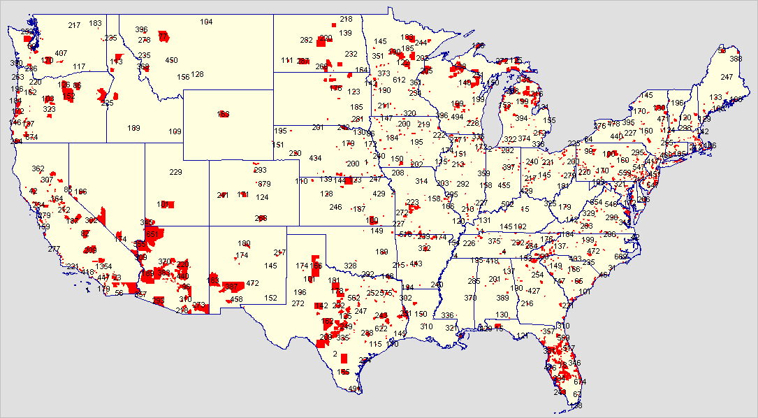
Naturally Occurring Retirement Communities, 2010
NORC areas are shown with a red fill pattern in the graphic presented below.

Click graphic for larger view labeled with number of NORC households.

A naturally occurring retirement community (NORC) is an area that naturally evolves over time to include a relatively large concentration of households where the householder is 65 years or older. NORCs evolve in or as neighborhoods generally on an unplanned basis. How are the more than 26 million households distributed as NORCs? How are they similar or dissimilar? What special needs do the population of some NORCs have compared to others? How will the evolvement of NORCs affect our society? This section is focused on U.S. national scope analysis of the size, distribution and characteristics of NORCs. Though unplanned, NORCs will continue to evolve as habitats that require decision-making information for planning. See extended detail in the related Web section.

Residents of NORCs may have requirements/needs that differ from other areas. These include transportation, social and education, assistance with household maintenance, healthcare and security. Demographics can help us assess the nature and magnitude of some of these needs and plan for improved solutions.

As of Census 2010, 25,819,836 households had a head of household age 65 years or over; 22.1% of total households. The Census 2010 U.S. size and distribution of households (occupied housing units) by age of head of householder is shown in the Summary File 1 Table 17 Tenure by Age of Householder. Using data from this table, households by tenure and different categories for age of head of household can be used in analyses.

Households: Tenure by Age of Householder
Total households: 116,716,292
  Owner occupied: 75,986,074
    Householder 15 to 24 years 869,610
    Householder 25 to 34 years 7,547,421
    Householder 35 to 44 years 13,255,629
    Householder 45 to 54 years 17,804,066
    Householder 55 to 59 years 8,626,564
    Householder 60 to 64 years 7,876,168
    Householder 65 to 74 years 10,834,028
    Householder 75 to 84 years 6,788,967
    Householder 85 years and over 2,383,621
  Renter occupied: 40,730,218
    Householder 15 to 24 years 4,531,189
    Householder 25 to 34 years 10,409,954
    Householder 35 to 44 years 8,035,251
    Householder 45 to 54 years 7,102,998
    Householder 55 to 59 years 2,701,749
    Householder 60 to 64 years 2,135,857
    Householder 65 to 74 years 2,670,489
    Householder 75 to 84 years 1,927,400
    Householder 85 years and over 1,215,331

NORCs & Block Group Demographics
Census block groups (BGs) are used to equivalence NORCs. Block groups average 1,500 in population and cover the U.S. wall-to-wall. Using a ProximityOne API, a dataset was developed containing the Census 2010 Table H17 data for each of the approximate 217,000 BGs. Those data were integrated into a national scope block group shapefile for mapping and geospatial analysis.

In 2010, 3.1 million households with head of household 65 years or over were located in 10,201 NORCs/BGs where the percent of head of households age 65 years and over is 40 percent or more. Each NORC/BG averages 307 households in this group.

Households versus Families
A family consists of two or more people (one of whom is the householder) related by birth, marriage, or adoption residing in the same housing unit. A household consists of all people who occupy a housing unit regardless of relationship. A household may consist of a person living alone or multiple unrelated individuals or families living together.

NORC Patterns and Visual Analysis
The illustrative views presented below were developed using the CV XE GIS software and NORC GIS project.

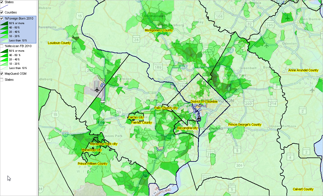
Washington, DC area NORCs, 2010 (red fill pattern)

Honolulu, HI area NORCs, 2010 (red fill pattern)

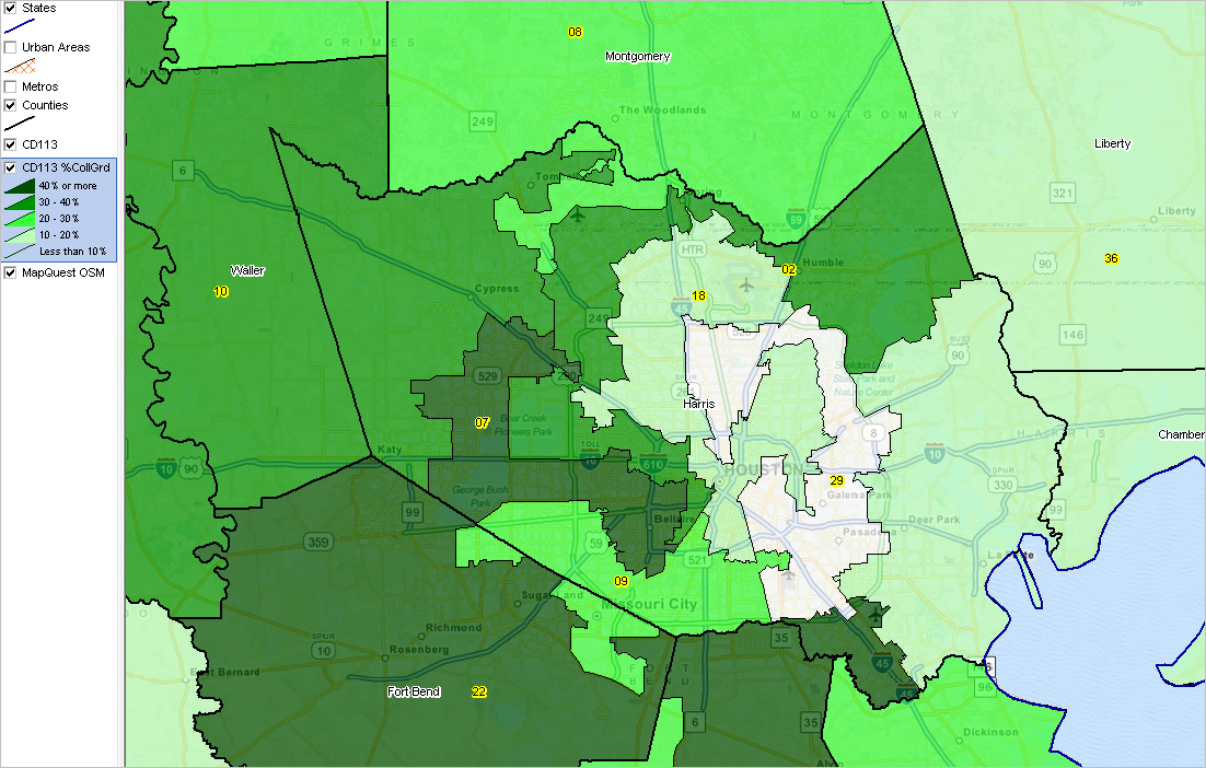
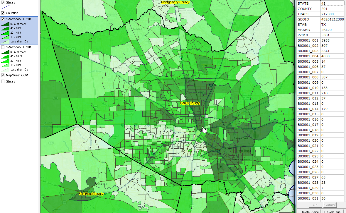
Houston, TX area NORCs, 2010 (red fill pattern)

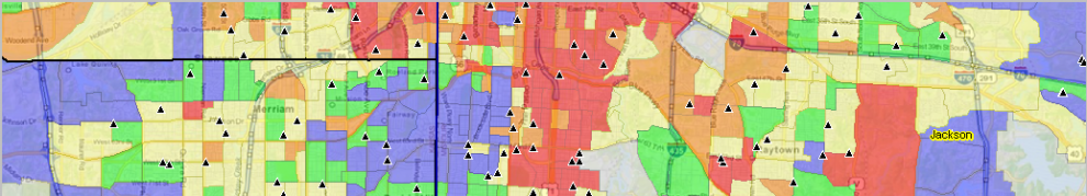
Kansas City, MO-KS area NORCs, 2010 (red fill pattern)
This view shows a mini-profile for a selected NORC (see pointer). The profile shows the 21 data field values from Census 2010 Summary File 1 Table H017 for this NORC/BG.

NORC Richer Demographics
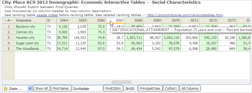
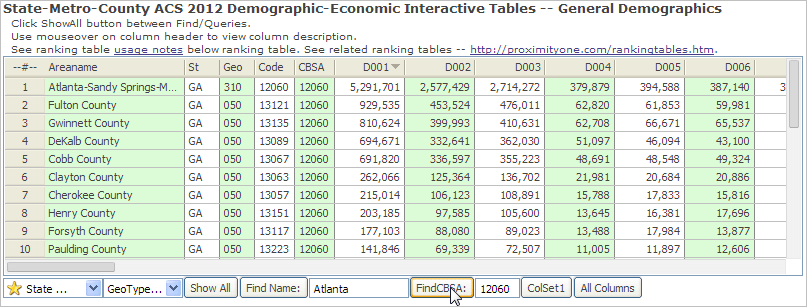
As of 2014, the Census 2010 demographics are the most up-to-date and accurate data available for block groups. The related American Community Survey (ACS) 5-year estimates are available at the block group level and provide “richer demographics” compared with data available through Census 2010. The 2012 ACS 5-year estimates (latest available until December 2014) are centric to mid-2010. The ACS 5-year estimates can provide insights into employment, income, poverty, language spoken, educational attainment, disabilities, among other relevant measures.

Join the ProximityOne User Group to use the NORC GIS project; view NORCs in context of other geography; add your own data; change colors, labeling, subject matter (join now, no fee).