Tip of the Day – Examining Median Housing Value – 2020 Update

.. tip of the day .. a continuing weekly or more frequent tip on developing, integrating, accessing and using geographic, demographic, economic and statistical data. Join in .. tip of the day posts are added to the Data Analytics Blog on an irregular basis, normally weekly. Follow the blog to receive updates as they occur.

.. in this era of uncertainly, we ponder the risk and opportunity associated with changing housing value.  Median housing value by ZIP Code area is one metric of great interest to examine levels and change.  While only one measure useful to examine housing characteristics, it is part of a broader set of demographic-economic data that enable analysis of the housing infrastructure and change in a more wholistic manner. How is housing value trending at the neighborhood level in 2020 and beyond? See more about the Situation & Outlook.

.. 5 ways to access/analyze the most recent estimates of median housing value and other subject matter by ZIP Code area .. based on the American Community Survey (ACS) 5-year estimates. See related Web section.

Option 1. View the data as a thematic pattern map
Option 1 is presented as Option 1A (using CV XE GIS) and Option 1B (using Visual Data Analytics VDA Mapserver). See more about GIS.

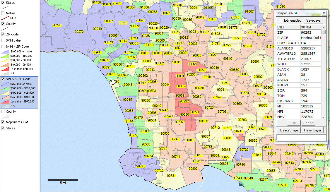
Option 1A. View $MHV as a thematic pattern map; using CV XE GIS:
— Median Housing Value by ZIP Code Area; Los Angeles Area
Click graphic for larger view with more detail.

Click graphic for larger view.
Use the Mapping ZIP Code Demographics resources to develop similar views anywhere in U.S.

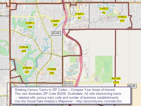
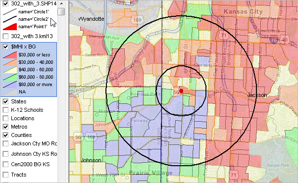
Option 1B. View $MHV (ACS 2018) as a thematic pattern map; using VDA Mapserver:
— Median Housing Value by ZIP Code Area; Phoenix/Scottsdale, AZ area
Click graphic for larger view with more detail.

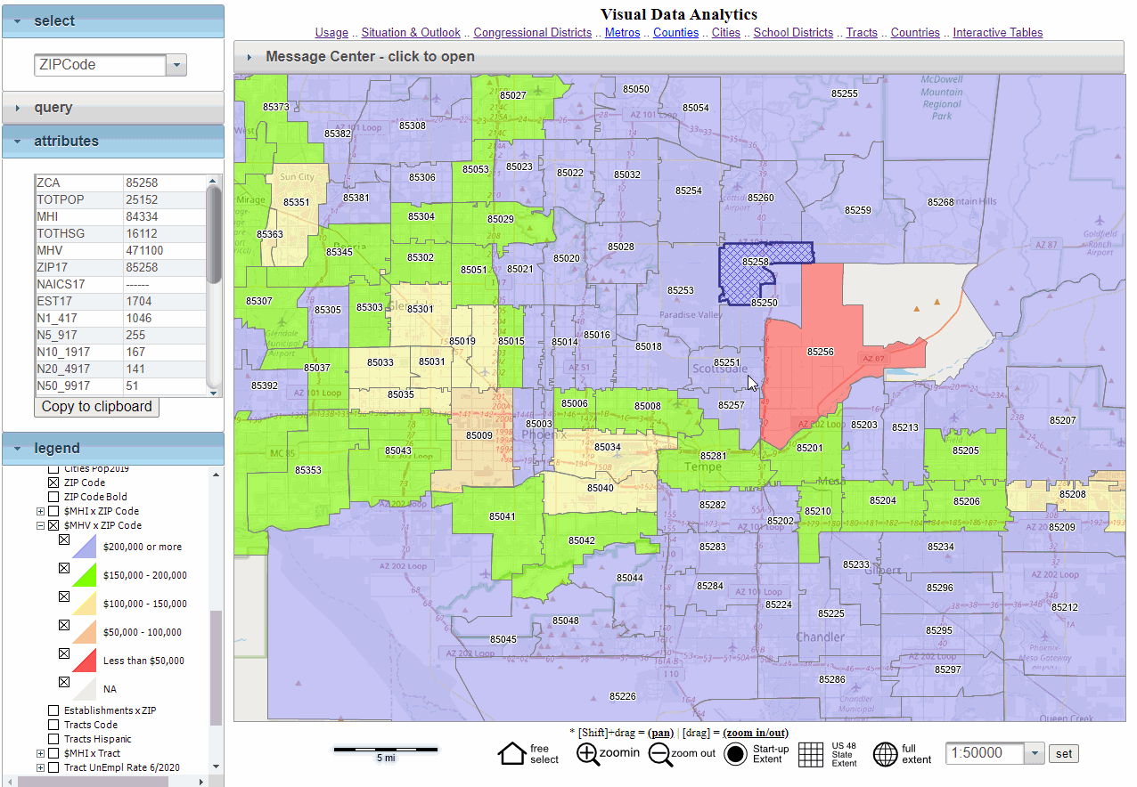
Click graphic for larger view. Expand window to full screen for best quality view. View features:
– profile of ZIP 85258 (blue crosshatch highlight) shown in Attributes panel at left
– values-colors shown in Legend panel at left
– transparency setting allows “see through” to view ground topology below.
Use VDA Mapserver: to develop similar views anywhere in U.S. using only a browser. Nothing to install.

Option 2. Use the interactive table:
– go to http://proximityone.com/zip18dp4.htm (5-year estimates)
– median housing value is item H089; see item list above interactive table.
– scroll left on the table until H089 appears in the header column.
– that column shows the 2018 ACS H089 estimate for for all ZIP codes.
– click column header to sort; click again to sort other direction.
– see usage notes below table.

Option 3. Use the API operation:
– develop file containing $MHV for all ZIP code areas in U.S.
– load into Excel, other software; link with other data.
– median housing value ($MHV) is item B25077_001E.
– click this link to get B25077_001E ($MHV) using the API tool.
– this API call retrieves U.S. national scope data.
– a new page displays showing a line/row for each ZIP code.
– median housing value appears on the left, then ZIP code.
– optionally save this file and import the data into a preferred program.
– more about API tools.
Extending option 3 … accessing race, origin and $MHV for each ZIP code …
click on these example APIs to access data for all ZIP codes
.. get extended subject matter for all ZIP codes
.. get extended subject matter for two selected ZIP codes (64112 and 65201)

Items used in these API calls:
.. B01003_001E – Total population
Age
.. B01001_011E — Male: 25 to 29 years (illustrating age cohort access)
.. B01001_035E — Female: 25 to 29 years (illustrating age cohort access)
Race/Origin
.. B02001_002E – White alone
.. B02001_003E – Black or African American alone
.. B02001_004E – American Indian and Alaska Native alone
.. B02001_005E – Asian alone
.. B02001_006E – Native Hawaiian and Other Pacific Islander alone
.. B02001_007E – Some other race alone
.. B02001_008E – Two or more races
.. B03001_003E – Hispanic (of any race)
Income
.. B19013_001E – Median household income ($)
.. B19113_001E – Median family income ($)
Housing & Households
.. B25001_001E – Total housing units
.. B25002_002E – Occupied housing units (households)
.. B19001_017E — Households with household income $200,000 or more
.. B25003_002E — Owner Occupied housing units
.. B25075_023E — Housing units value $500,000 to $749,999
.. B25075_024E — Housing units with value $750,000 to $999,999
.. B25075_025E — Housing units with value $1,000,000 or more
.. B25002_003E – Vacant housing units
.. B25077_001E – Median housing value ($) – owner occupied units
.. B25064_001E – Median gross rent ($) – renter occupied units

View additional subject matter options.

Option 4. View the $MHV in context of other attributes for a ZIP code.
Using – ACS demographic-economic profiles. Example for ZIP 85258:
– General Demographics ACS 2018 .. ACS 2017
– Social Characteristics ACS 2018 .. ACS 2017
– Economic Characteristics ACS 2018 .. ACS 2017
– Housing Characteristics ACS 2018 .. ACS 2017 .. $MHV shown in this profile.

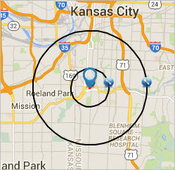
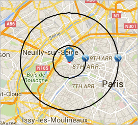
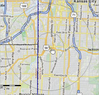
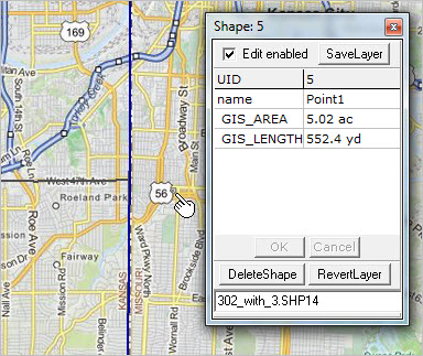
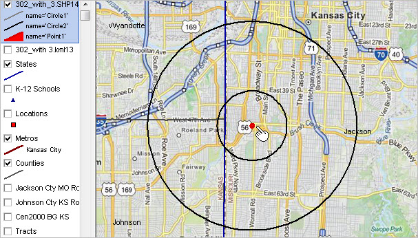
Option 5. View 5- and 10-mile circular area profile from ZIP center.
– profile for ZIP 80204 dynamically made using SiteReport tool.
– with SiteReport running, enter the ZIP code, radii and click Run.
– comparative analysis report is generated in HTML and Excel structure.
– Click this link to view resulting profile.
– from the profile, site 2 is 1.9 times the population of site 1.
– Site 1 $MHV is $296,998 compared to Site 2 $MHV $269,734.
– GIS view with integrated radius shown below.

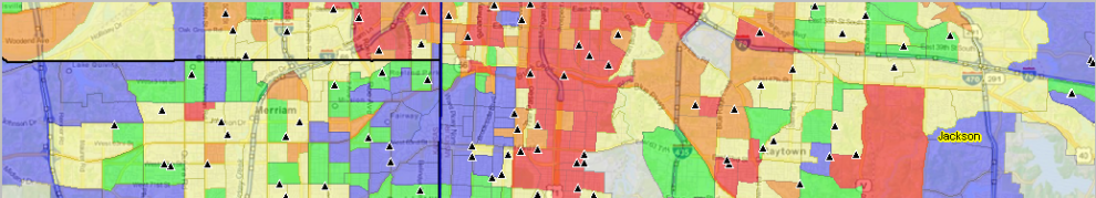
This section is focused on median housing value and ZIP code areas. Many other subject matter items will be apparent when these methods are used. Optionally adjust above details to view different subject matter for ZIP codes.

Join me in a Data Analytics Lab session to discuss more details about accessing and using wide-ranging demographic-economic data and data analytics. Learn more about using these data for areas and applications of interest.

About the Author
— Warren Glimpse is former senior Census Bureau statistician responsible for innovative data access and use operations. He is also the former associate director of the U.S. Office of Federal Statistical Policy and Standards for data access and use. He has more than 20 years of experience in the private sector developing data resources and tools for integration and analysis of geographic, demographic, economic and business data. Contact Warren. Join Warren on LinkedIn.

VDA Mapserver: Comparing Census Tracts & ZIP Codes

.. for small area demographic-economic analysis, census tracts and ZIP code areas both have their advantages and disadvantages.  While the same scope of subject matter data are available from the American Community Survey (ACS) and ProximityOne current estimates and projections for these geographies, it can be difficult to view how the geographic areas visually relate or intersect in a map.  A flexible solution, accessible by any Web browser, is the Virtual Data Analytics (VDA) Mapserver.  See details.  You can start using VDA immediately with nothing to install.

Visual Data Analytics Mapserver
The VDA Mapserver is a learning resource, a tool that you can use for interactive mapping and geospatial analysis using only Internet and a browser. The VDA Mapserver is set apart from related tools due to the scope and style of accessing data for wide-ranging geography and frequently updated demographic-economic subject matter data. Use the unique combination of Federal statistical data with proprietary current estimates and projections.

Other geographies and subject matter will be reviewed in subject posts.

An Illustration: ZIP Code Area 85258, Scottsdale, AZ

– click for larger view.

The above shows a zoom-in to ZIP code area 85258 in Scottsdale, AZ. A step-by-by description of how to develop this view is shown in this section of the VDA guide.

As shown in the graphic, ZIP Code area 85258 intersects with 8 census tracts. ZIP code areas and tracts are not coterminous. On average there are approximately 2.5 tracts per ZIP code area. But there are more than 150,000 intersecting combinations of ZIP Code areas and tracts. See intersecting areas and interactive table.

Learn more — Join me in the Situation & Outlook Web Sessions
Join me in a Situation & Outlook Web Session where we discuss topics relating to measuring and interpreting the where, what, when, how and how much demographic-economic change is occurring and it’s impact.

About the Author
— Warren Glimpse is former senior Census Bureau statistician responsible for national scope statistical programs and innovative data access and use operations. He is also the former associate director of the U.S. Office of Federal Statistical Policy and Standards for data access and use. He has more than 20 years of experience in the private sector developing data resources and tools for integration and analysis of geographic, demographic, economic and business data. Contact Warren. Join Warren on LinkedIn.

Census 2020 Residential Address Counts by Block

.. using Census 2020 residential address count data to examine change since 2010 .. the Census Bureau has released preliminary Census 2020 residential address counts by Census 2010 census block. These data, count of residential addresses and group quarters addresses, reflect updates as of October 2019 and do not represent final Census 2020 counts. The data will continue to be updated to support Census 2020. See related Web section with more detail and updates.

Importance and Use
These data are of immediate value in determining and analyzing how the number of housing units have changed, 2010 to 2019. Since the data are at the census block level, they may be aggregated to any other Census-defined summary level/type of geographic area such as block group, tract, ZIP code, city, county, school district, etc. These data are also important as they give us a “year in advance look” at how small area demographics are changing since 2010. Before this, the most recent census block data were from Census 2010. A lot has happened in many areas. These data provide insights into that change. The Census 2020 block level data will be released in early 2021 for Census 2020 census block geography. So, another important feature of these data is that they are summarized for Census 2010 census block boundaries. Census 2010 and 2020 block boundaries may differ, particularly in areas experiencing larger demographic growth/change. An important limitation is that they are counts, subject to change as the Census data are collected/tabulated.

Comparing Census 2010 Housing Units with Census 2020 Address Counts
The following graphic shows patterns of Census 2010 housing counts with the Census 2020 (late 2019 vintage) residential address counts by census block. This view is focused on census tract 3608100700 (tract 000700) in Queens County, NY (code shown near center of graphic). Individual blocks are labeled with block code (4 digits) with the Census 2010 housing units (yellow label) and Census 2020 residential address count (green label) shown below the block code. As an example, the block located at the pointer has block code 3006 (or full national scope unique block code 36-081-00700-3006) with a Census 2010 count 44 housing units and a Census 2020 (late 2019 count) of 232 residential addresses. Click graphic for larger view. Expand browser window to full screen for best quality view.

.. view created with ProximityOne CV XE GIS software and related GIS project.

More About Using these Data
We have summarized these data at the census tract level and are evaluating their use, in combination with other data, to develop current estimates and projections to 2025.

Data Analytics Web Sessions
Join me in a Demographics Analytics Lab session to discuss more details about accessing and using wide-ranging demographic-economic data and data analytics. Learn more about using these data for areas and applications of interest.

About the Author
— Warren Glimpse is former senior Census Bureau statistician responsible for innovative data access and use operations. He is also the former associate director of the U.S. Office of Federal Statistical Policy and Standards for data access and use. He has more than 20 years of experience in the private sector developing data resources and tools for integration and analysis of geographic, demographic, economic and business data. Contact Warren. Join Warren on LinkedIn.

Using GIS & GeoDemographics

.. join us in the GIS & GeoDemographics self-paced, online course.

Visual representation, maps, of demographic data by geographic area can be exciting and rewarding. Using Geographic Information Systems (GIS) can bring maps alive. Creativity is boundless. The banner at the top of the corresponding Web section presents a static view of a map rendered using GIS. This map shows the Los Angeles area by census tract. For the analyst or stakeholder, it shows something more — the percent Asian citizen voting age population by tract, overlayed with Congressional District boundaries and codes. It shows relationships, patterns. Using the power of GIS, the zoom level, colors, legend, and labeling can all be changed immediately. You, the GIS user, are at once analyst, artist and storyteller. In control of your medium, canvas, you further your benefits from use these software and data by making dynamic presentations in collaborations. Make compelling arguments. Capture your views and blend them with words and charts into documents. Welcome to the world of GIS and geodemographics.

Mapping census block demographics
The graphic shown below illustrates use of GIS software with the TIGER digital map database census block shapefile to show census blocks for two Ohio counties in context of 2018 CBSAs/Metros. Clicking on a census block (see pointer) shows a mini profile for that block.

– view developed using ProximityOne CV XE GIS and related GIS project.

Using GIS & GeoDemographics .. about the course
Examining geographic-demographic-economic characteristics, patterns and trends … researchers, policymakers, journalists, administrators, students among others. How can you most benefit from using the TIGER geographic data to meet your objectives? These data are available at no cost. Join us in the Using GIS Tools & GeoDemographics online, self-paced course. Learn all aspects of using the Census Bureau TIGER files and related Census-sourced and other Federal statistical data. Augment your professional skills; participants receive all required data, methods and tools. Your personal session is developed and coordinated by Warren Glimpse. You receive the GIS course certificate upon completion. The course may be started at any time and includes requisite Windows-based CV XE GIS software. The course assumes the participant has basic familiarity with a Windows computer, Internet and spreadsheet operations. No GIS related experience is required. Experienced GIS professionals also benefit by learning about the use and nuances of Census-sourced data and integrating these with other data. The structure includes four segments that typically require 2.5 hours each. It is feasible to complete the course in a day or two though we suggest two weeks.

Use Geographic Information Systems (GIS) with TIGER … integrate/analyze data from American Community Survey (ACS) or the decennial census (Census 2010) (Census 2020) into TIGER files to make thematic maps. Merge data from other statistical programs. Geocode your address-based data and add the geocoded data to a GIS project/map view; examine patterns. View your market/service areas and assess competitive position, unmet opportunities. Learn about procedures and strategies to develop GIS projects that meet your needs. Acquire the tools and data to perform these tasks without spending more — provided as a part of our course.

The course is not just about TIGER and demographic-economic data. It provides a well-rounded framework for how to use GIS. While TIGER is a focus, we review procedures to access and use thousands of public use shapefiles and GIS files that may be useful to you. It provides a well-rounded framework for how to use GIS.

Enroll today …
Click the enrollment button/link (opens new page) to enroll now ($395). We will contact you and provide next step information.   Questions? Call us at (800)364-7656.

Data Analytics Web Sessions
Join me in a Demographics Analytics Lab session to discuss more details about accessing and using wide-ranging demographic-economic data and data analytics. Learn more about using these data for areas and applications of interest.

About the Author
— Warren Glimpse is former senior Census Bureau statistician responsible for innovative data access and use operations. He is also the former associate director of the U.S. Office of Federal Statistical Policy and Standards for data access and use. He has more than 20 years of experience in the private sector developing data resources and tools for integration and analysis of geographic, demographic, economic and business data. Contact Warren. Join Warren on LinkedIn.

Census Tract Demographic-Economic Characteristics & Trends

..  Census tract demographics are used in wide-ranging public and private sector applications to examine patterns and characteristics of sub-county areas. Tract level data from Census 2000, Census 2010 and the American Community Survey (ACS) can be used to analyze trade/market areas, neighborhoods and other small area study areas. But what about more current data and trends since 2010? What about business establishment data and other subject matter not included in either the census or ACS data?

There are no current demographic-economic census tract data available from the Census Bureau or other Federal statistical programs. Annually released ACS 5-year estimates are available by census tract but are for 5-year periods and dated. The most recent census tract level ACS data are based on the ACS 2017 5-year estimates (ACS 1317). Those data are not for the year 2017 but estimates for ACS survey respondents for the 5 year period 2013-2017; centric to mid-2015.

Patterns of Median Household Income %Change by Census Tract
The graphic below shows patterns of economic prosperity change based on median household income percent change ACS 2012 to ACS 2017 by tract in the Dallas metro area.

– view developed using ProximityOne CV XE GIS and related GIS project.

Using the Interactive Table
Use the interactive table .. click this link .. to view, query, rank, compare selected characteristics of the population, housing, educational attainment and income for census tracts based on ACS 2012 5-year, and ACS 2017 5-year data. Hundreds of additional items are available. See about related census tract data resources and applications.

Try it yourself ..
Tracts with ACS 2017 population 3,500-4,500 ranked on change in $MHI:
Replicate the following graphic using the interactive table. This view was produced by clicking the Pop17 button below the table to select only tracts with a ACS 2017 population between 3,500 and 4,500. Then the $MHI columns button was clicked to view only selected columns. Finally the qualifying tracts were sorted in descending order by clicking the $MHI Change column header cell.

Based on these estimates, tract 04013105004 in Maricopa County, AZ is top ranked, where the $MHI increased by $97,723 from the ACS 2012 5-year period to the ACS 2017 5-year period.

Corresponding API calls to access the $MHI for this tract (click links to access data):
ACS 2012 $MHI … ACS 2017 $MHI
Join us in an upcoming Data Analytics Web Session (see below) to learn more about using APIs to access these data and similar data.

Access more detailed ACS 2017 tract interactive tables:
  General demographics .. Social .. Economic .. Housing

Demographic Analytics Web Sessions
Join me in a Demographics Analytics Lab session to discuss more details about accessing and using wide-ranging demographic-economic data and data analytics. Learn more about using these data for areas and applications of interest.

About the Author
— Warren Glimpse is former senior Census Bureau statistician responsible for innovative data access and use operations. He is also the former associate director of the U.S. Office of Federal Statistical Policy and Standards for data access and use. He has more than 20 years of experience in the private sector developing data resources and tools for integration and analysis of geographic, demographic, economic and business data. Contact Warren. Join Warren on LinkedIn.

Creating Custom School District Maps

…tools & data to map & geospatially analyze school districts. Ready-to-use state-by-state GIS projects may be downloaded enabling you to view and create custom maps almost instantly. Benefit from the power of using GIS software to perform tasks not available on Web-based mapping options. Use the latest school district and related shapefiles. See more information about using these resources in this related Web section.

Federal Revenue per Student by School District
Create views similar to the one shown below. Optionally combine layers as illstrated here by showing four Texas metros.

.. view developed with CV XE GIS and related GIS project.

Extending Reference and Analytical Possibilities

Texas by School District
Examine reference maps at the state, regional or local level. Optionally combine with roads/streets and other layers.

Patterns of Economic Prosperity by School District
Select from many ready-to-use demographic-economic subject matter items to create custom pattern views.

Drill-down — Houston Metro Area by School District
Zoom-in to a school district of interest. Set attributes of district as shown here.
–

County/School District
Visually examine the boundaries or school districts and counties. This view shows Harris County, TX area; select a county of interest.

Drill-down to Street Level
Add road/street and other layers. Drill-down within Fort Bend ISD, Houston metro, showing general earth surface features with streets layers. Mouse used to click on street (see pointer) and display mini-profile of street segment attributes.

Use for Analysis, Reference or in the Classroom
Schools and teachers: consider using these resources for classroom use. Familiarize students about how GIS resources can be used with a minimum of learning time and no cost. Enable students to use their own geography and adapt that learning to more general geography. See related Mapping Statistical Data ready-to-use GIS projects.

Join me in a Data Analytics Lab session to discuss more details about accessing and using wide-ranging demographic-economic data and data analytics. Learn more about using these data for areas and applications of interest.

About the Author
— Warren Glimpse is former senior Census Bureau statistician responsible for innovative data access and use operations. He is also the former associate director of the U.S. Office of Federal Statistical Policy and Standards for data access and use. He has more than 20 years of experience in the private sector developing data resources and tools for integration and analysis of geographic, demographic, economic and business data. Contact Warren. Join Warren on LinkedIn.

Developing Geographic Relationship Data

.. tools and methods to build and use geographic relationship files … which census blocks or block groups intersect with one or a set of school attendance zones (SAZ)? How to determine which counties are touched by a metropolitan area? Which are contained within a metropolitan area? Which pipelines having selected attributes pass through water in a designated geographic extent? This section reviews use of the Shp2Shp tool and methods to develop a geographic relationship file by relating any two separate otherwise unrelated shapefiles. See relasted Web page for a more detiled review of using Shp2Shp.

As an example, use Shp2Shp to view/determine block groups intersecting with custom defined study/market/service area(s) … the only practical method of obtaining these codes for demographic-economic analysis.

– the custom defined polygon was created using the CV XE GIS AddShapes tool.

Many geodemographic analyses require knowing how geometries geospatially relate to other geometries. Examples include congressional/legislative redistricting, sales/service territory management and school district attendance zones.

The CV XE GIS Shape-to-Shape (Shp2Shp) relational analysis feature provides many geospatial processing operations useful to meet these needs. Shp2Shp determines geographic/spatial relationships of shapes in two shapefiles and provides information to the user about these relationships. Shp2Shp uses the DE-9IM topological model and provides an extended array of geographic and subject matter for the spatially related geometries. Sh2Shp helps users extend visual analysis of geographically based subject matter. Examples:
• county(s) that touch (are adjacent to) a specified county.
• block groups(s) that touch (are adjacent to) a specified block group.
• census blocks correspond to a specified school attendance zone.
• attributes of block groups crossed by a delivery route.

Block Groups that Touch a Selected Block Group
The following graphic illustrates the results of using the Shp2Shp tool to determine which block groups touch block group 48-85-030530-2 — a block group located within McKinney, TX. Shp2Shp determines which block groups touch this block group, then selects/depicts (crosshatch pattern) these block groups in the corresponding GIS map view.

Geographic Reference File
In the process, Shp2Shp creates a geographic relationship file as illustrated below. There are six block groups touching the specified block group. As shown in the above view, one of these block groups touches only at one point. The table below (derived from the XLS file output by Shp2Shp) shows six rows corresponding to the six touching block groups. The table contains two columns; column one corresponds to the field GEOID from Layer 1 (the output field as specified in edit box 1.2 in above graphic) and column 2 corresponds to the field GEOID from Layer 2 (the output field as specified in edit box 2.2 in above graphic). The Layer 1 column has a constant value because a query was set (geoid=’480850305302′) as shown in edit box 1.3. in the above graphic. Any field in the layer dataset could have been chosen. The GEOID may be used more often for subsequent steps using the GRF and further described below. It is coincidental that both layers/shapefiles have the field named “GEOID”.

Layer 1	Layer 2
480850305302	480850305272
480850305302	480850305281
480850305302	480850305301
480850305302	480850305311
480850305302	480850305271
480850305302	480850305312

Note that in the above example, only the geocodes are output for each geography/shape meeting the type of geospatial relationship. Any filed within either shapefile may be selected for output (e.g., name, demographic-economic field value, etc.)

How it Works — Shp2Shp Operations
The following graphic shows the settings used to develop the map view shown above.

See related section providing details on using the Shp2Shp tool.

Geographic Relationships Supported
The Select Relationships dropdown shown in the above graphic is used to determine what type of spatial relationship is to be used. Options include:
• Equality
• Disjoint
• Intersect
• Touch
• Overlap
• Cross
• Within
• Contains
See more about the DE-9IM topological model used by Shp2Shp.

Try it Yourself

See full details on how you can use any version, including the no fee versin, of CV XE GIS to use the Shp2Shp tools. Here are two examples what you can d. Use any of the geospatial relatoinships. Apply your own queries.

Using Touch Operation
Select the type of geographic operation as Touch. Click Find Matches button. The map view now shows as:

Using Contains Operation
Click RevertAll button. Select the type of geographic operation as Contains. Click Find Matches button. The map view now shows as:

Relating Census Block and School Attendance Zones
The graphic shown below illustrates census blocks intersecting with Joyner Elementary School attendance zone located in Guilford County Schools, NC (see district profile). The attendance zone is shown with bold blue boundary. Joyner ES SAZ intersecting blocks are shown with black boundaries and labeled with Census 2010 total population (item P0010001 as described in table below graphic). Joyner ES is shown with red marker in lower right.

– view developed using CV XE GIS and related GIS project; click graphic for larger view

See more about this application in this related Web section.

Join me in a Data Analytics Lab session to discuss more details about accessing and using wide-ranging demographic-economic data and data analytics. Learn more about using these data for areas and applications of interest.

About the Author
— Warren Glimpse is former senior Census Bureau statistician responsible for innovative data access and use operations. He is also the former associate director of the U.S. Office of Federal Statistical Policy and Standards for data access and use. He has more than 20 years of experience in the private sector developing data resources and tools for integration and analysis of geographic, demographic, economic and business data. Contact Warren. Join Warren on LinkedIn.

Mapping Census Tract Demographics

.. using visual data analytics and developing business intelligence .. this section provides a 4-step procedure to develop thematic pattern and reference maps for census tracts. The focus of this section is on mapping Census 2010 census tracts using data from the 2014 American Community Survey (ACS2014). A similar set of steps could be followed for Census 2000 tracts with Census 2000 data or Census 2010 tracts with Census 2010 demographics or different vintage ACS data. Steps summarized here can be used with most any Windows-based computer having Internet access. See the related full Web section with more details.

• how do customers and sales relate to market area characteristics?
• is their a better configuration of locations or service areas?
• how can you more effectively examine customer and sales patterns?
• what and where are areas of missed opportunities?

See related sections:
• Using GIS & Data Analytics
• Mapping Statistical Data

Benefits of this section include providing help for those:
• having a specific interest in mapping census tract demographics.
• with little or no experience in using GIS.
• getting started with CVGIS.

These resources and instructions provide a real, not demo, valuable tool that anyone can use, without fee, to create county by census tract thematic pattern maps. Use any of the “richer” demographic-economic data (not just median household income) from the latest ACS 5-year data (see scope — table shells xls).

The steps described below can be performed with any version of CVGIS, including the no fee version. Start from scratch and develop thematic pattern maps like that shown below. Questions, need help? See the FAQs. Call with questions – 888.364.7656. Or, use this form and put questions in the text section.

While this application is focused on ACS 2014 median household income for Dallas County, TX census tracts, you can follow these steps for other areas and subject matter. In your own applications, choose any ACS subject matter for any county/area of interest. The following view shows the end result of steps described below. Choose your own county of state; choose your own subject matter; select your own colors and labeling; choose your own zoom view; and more. Dallas Metro Situation & Outlook.

Patterns of Economic Prosperity; Dallas County, TX by Tract

Mapping Census Tracts Demographics Steps
These steps should take an inexperienced user 10-15 minutes to develop a new CVGIS project view. Steps can be performed at separate times.
Click on a link to view step-by-step instructions.
1. Install CVGIS
2. Get census tract shapefile
3. Get census tract subject matter data (median household income or other)
4. Create map view(s)

Create your own maps for your own county/tracts for your own subject matter.

Join me in a Data Analytics Lab session to discuss more details about accessing and using wide-ranging demographic-economic data and data analytics. Learn more about using these data for areas and applications of interest.

About the Author
— Warren Glimpse is former senior Census Bureau statistician responsible for innovative data access and use operations. He is also the former associate director of the U.S. Office of Federal Statistical Policy and Standards for data access and use. He has more than 20 years of experience in the private sector developing data resources and tools for integration and analysis of geographic, demographic, economic and business data. Contact Warren. Join Warren on LinkedIn.

Developing & Using Map Graphics

.. steps to develop map graphics & visual analysis of market/study areas .. map graphics are an important part of most demographic-economic analyses and essential for many applications. Not only are are maps needed to show geographic boundaries and the relative location of geography within a broader area, they can come alive by showing patterns. A thematic pattern map of median household income by block group is a good example; higher and lower areas of economic prosperity by neighborhood can be immediately determined. Map graphics can improve our ability to communicate complex information. Convey information faster. Make more compelling presentations. Collaborate more effectively through the use of map graphics.  See related Web section for more details.

The focus of this section is on creating and using KML files to prepare map graphics for use in developing Market-Study Area Comparative Analysis Reports. These files and map graphics also have broader uses. Steps are reviewed to develop the KML circular area map graphics files, convert them to shapefile structure and integrate both files into mapping and GIS applications and put them into operational use. 

KML (Keyhole Markup Language) files are XML structured files useful for visualizing geographic objects (like circles) using Internet-based browsers, notably Google Earth. Why develop/use KML files? They are easy to create with precision, there is little to no learning curve, they can be used in many venues and they are free to develop. KML files can be used side-by-side with shapefiles. Shapefiles, structured very much unlike KML files, are the dominant vector-based file structure used in GIS applications involved in both viewing and geospatial analysis. 

Developing Circular KML Files & Map Graphics
An “objective view” of this section is shown in the following graphic. The graphic shows a study site location (red marker), 1-mile & 3-mile radius circles. The site location is a Starbucks located at 302 Nichols Road, Kansas City, MO 64112. The view shows a circular KML-based graphics in context of patterns of median household income by block group. Develop similar views for any area, any site circular configuration, using steps reviewed in this section.

– view developed using CV XE GIS

Creating the KML Circular Graphics File
Proceed through the next steps to develop a KML file used to create the graphic below on left — a Starbucks located at 302 Nichols Road, Kansas City, MO 64112. Graphic on the right is a Starbucks location in Paris, used to illustrate this process works globally. Both graphics include study area center point and 1-mile and 3-mile radius circles.

302 Nichols Road, Kansas City, MO 64112

23 Avenue de Wagram, 75001 Paris, France

Start the create KML file application
• Key in address 302 Nichols Road, Kansas City, MO 64112 to Google Maps
.. see the latitude-longitude (39.041548,-94.592965) in the URL bar.
• Open this web page to create the circles & save results as KML file.
• Refresh this page if making a new KML file.
• Set the colors and lines to medium, blank and clear.
• Enter coordinates — key in lat 39.041548 and lon -94.592965
.. these for for this example
.. enter the values for your location of interest
Add center point
• In the Radius Distance, key in 0.05 miles
• Click Draw Radius blue button (at right of longitude).
Add site 1 circle
• In the Radius Distance, key in 1.00 miles (use preferred radius for inner circle).
• Click Draw Radius blue button (at right of longitude).
Add site 2 circle
• In the Radius Distance, key in 3.00 miles (use preferred radius for inner circle).
• Click Draw Radius blue button (at right of longitude).
View study area geography
• Optionally navigate up to the map view and make the view similar to the graphic at the top of this page 
.. this step is not required but might be useful to verify the study area appearance.
Save KML file
• Navigate down the page to “Google Earth KML Output”. Click the blue button Generate KML.
• Click “Download KML file Here.” Save the file to a folder and make a note of the file path and name
.. save the file as c:\sitereport\302nichols.kml (this file and filename are used below).
Done
• The three part KML file has been created and saved to the local computer. 
• Finished using this browser application.

This same process may be used again to create similarly structured KML files of any radius about any point for any location in the world. 

Loading a KML file into Google Maps
Optionally create the objective map graphic using the following steps. Or, the KML file may be used with the CV XE GIS software (see below) enabling yet further analytical possibilities. 

• Click this link to start the Google MyMaps application.
• When the new page opens click create new map button
• Next click import button
• Enter the file path/name as created above (c:\sitereport\302nichols.kml), or any KML file.
• Edit the MyMaps rendering to achieve preferred view.
• Use preferred screen capture tool to save that part of the map view as a graphic for the study report.

Using the KML File with an Existing GIS Project and converting the KML file to shapefile structure

1. Add the KML file to an Existing CV XE GIS Project
• Start the CV XE GIS software and open the project file c:\cvxe\1\cvxe_us2.gis (distributed with installer).
.. uncheck Locations and $MHI x BG layers in legend panel.
• Click the AddLayer button (second button from left on toolbar)
• Select the KML file that was created above (c:\sitereport\302nichols.kml) .. circles appear in the map window.
• Use LayerEditor to adjust settings for KML layer (transparent, bold outline)
• Navigate to zoom-in view and smaller map window.
• Use Toolbar button Save to Image (button 7 from left) to save the map window view to a .jpg file.

Navigate to this view:

2. Converting a KML File to a Shapefile
This step requires the CV XE GIS Basic or higher level version. After the KML layer appears in the above sequence, proceed as follows:

• Click File>ExportShapefile.
• Select the KML layer name.
• Set Coordinate System edit box value to NAD83.
• Click OK button.
• On the Export Layer/FileSave dialog, select an output file path and name.
• The shapefile is generated and may be reused with any GIS project.

3. Editing attributes of the study area shapefile and project file
There are three shapes in the shapefile (center point, circle 1, circle 2). 
Modify the appearance of these shapes/objects by using the Select tool (mouse in Select mode).
• In legend panel click on circles layer; name turns blue indicating this is the active layer.
• In the map window, click in the circle; the profile/editor appears (pop-up)
• Initially all three shapes have the name “Polygon”.
.. change the object names successively to Point1 (the small circle), Circle1 and Circle2.
• The shapefile attributes have been permanently changed.
• When each shape/object has been renamed, use the LayerEditor to modify the appearance of each shape.
.. the changes modify the project file and not the shapefile.
.. optional save the project (overwriting the former version) or save the project with a new name.

Renaming a shape to “Point1”
Click for larger view

Using LayerEditor to set attributes of the study area layer
Click for larger view

View of final study area layer in context of broader project
Click for larger view

View as above with $MHI x BG checked on/visible
Click for larger view
 

Join me in a Data Analytics Lab session to discuss more details about accessing and using wide-ranging demographic-economic data and data analytics. Learn more about using these data for areas and applications of interest.

About the Author
— Warren Glimpse is former senior Census Bureau statistician responsible for innovative data access and use operations. He is also the former associate director of the U.S. Office of Federal Statistical Policy and Standards for data access and use. He has more than 20 years of experience in the private sector developing data resources and tools for integration and analysis of geographic, demographic, economic and business data. Contact Warren. Join Warren on LinkedIn.

Relating Block Groups to ZIP Code Areas

.. the popularity of block group demographic data is mainly due to this being the smallest geographic area for which annually updated demographic data, with U.S. wall-to-wall coverage, are available from the American Community Survey (ACS) — or any other source. While block groups nest within census tracts from both a geometric and geocode hierarchy perspective, the relationship between block groups and ZIP code areas is far less clear. Analysts are often interested in relating block group geography and demographics with ZIP code areas. The Census 2010 217,740 block groups intersect with 32,824 ZIP code areas forming 308,805 BG-ZIP area combinations. This section reviews tools to examine the relationship between block group geography/demographics and ZIP code areas. See related Web section for full details.

Block Group 06-075-015700-1 in Context of ZIP Code Area 94115
Block groups (BGs) are often wholly contained within a ZIP code area. But around the ZIP code area boundary, intersecting block groups are often split by the ZIP code boundary. This relationship is illustrated in the graphic shown below. This graphic shows block group 06-075-015700-1 (yellow BG code label, cross-hatched, black boundary) in context of ZIP Code area 94115 (white labels, bold blue boundary) located in San Francisco. This GIS application is closely related to the Mapping Block Group Data, also uses the San Francisco area in applications.

– view developed with ProximityOne CV XE GIS and related GIS project.
– view all San Francisco ZIP code areas; see ZIP 94115 in context.

The cross-hatched BG 060750157001 (or 06-075-015700-1) is split by ZIP code 94115. What part of the BG is in ZIP code area 94115 and adjacent ZIP code area 94118? The situation is similar for BG 060750157002, directly below 060750157001, which is split into 3 ZIP code areas. Use the interactive table to make these determinations.

Using the Interactive Table
The interactive table illustrated in the graphic below contains a row for block group area part which intersects with a unique ZIP code area. The simple case of a BG being split into two ZIP code areas can be visually observed as shown in the graphic presented above. A tabular relational table offers processing advantages compared to visual geospatial depictions. Here is an example. ZIP code area 94115 contains whole or parts of 32 BGs. To view/verify this using the table below, 1) click the ShowAll button below the table, then 2) click the Find ZIP button (edit box at right preloaded with this ZIP). The table refreshes with 32 rows — the BGs intersecting with this ZIP code area. Verify there are 32 BGs; the BG codes can be viewed in column 1.

In the above map at the top of this section, block group 06-075-015700-1 is shown visually to be contained in two ZIP code areas. To view how block group 06-075-015700-1 is split among multiple ZIP code areas using the table below, 1) click the ShowAll button below the table, then 2) click the Find GEOID button (enter G0607501057001 in the edit box to right of Find GEOID then click Find button). The table refreshes with two BGs. In this example, it can be seen that the total BG population (Census 2010) is 1,375. The part of the BG population is shown and the percent of the population from that BG allocated to the corresponding ZIP code are shown. This BG has a total area 0.09 square miles. The part of the BG area Census 2010, square miles) is shown and the percent of the area from that BG allocated to the corresponding ZIP code are shown.

Use the main Web section interactive table to examine areas of interest. Join me in a Data Analytics Lab session to discuss use of these data using analytical tools and methods applied to your situation.

About the Author
— Warren Glimpse is former senior Census Bureau statistician responsible for innovative data access and use operations. He is also the former associate director of the U.S. Office of Federal Statistical Policy and Standards for data access and use. He has more than 20 years of experience in the private sector developing data resources and tools for integration and analysis of geographic, demographic, economic and business data. Contact Warren. Join Warren on LinkedIn.