.. tools and methods to build and use geographic relationship files … which census blocks or block groups intersect with one or a set of school attendance zones (SAZ)? How to determine which counties are touched by a metropolitan area? Which are contained within a metropolitan area? Which pipelines having selected attributes pass through water in a designated geographic extent? This section reviews use of the Shp2Shp tool and methods to develop a geographic relationship file by relating any two separate otherwise unrelated shapefiles. See relasted Web page for a more detiled review of using Shp2Shp.
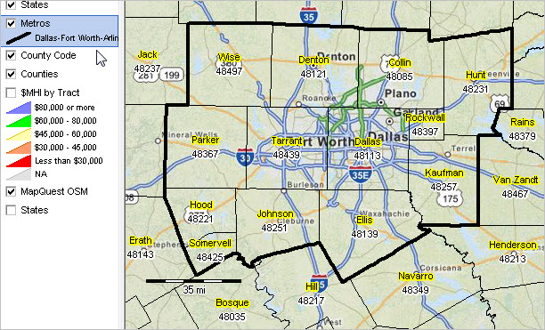
As an example, use Shp2Shp to view/determine block groups intersecting with custom defined study/market/service area(s) … the only practical method of obtaining these codes for demographic-economic analysis.

– the custom defined polygon was created using the CV XE GIS AddShapes tool.
Many geodemographic analyses require knowing how geometries geospatially relate to other geometries. Examples include congressional/legislative redistricting, sales/service territory management and school district attendance zones.
The CV XE GIS Shape-to-Shape (Shp2Shp) relational analysis feature provides many geospatial processing operations useful to meet these needs. Shp2Shp determines geographic/spatial relationships of shapes in two shapefiles and provides information to the user about these relationships. Shp2Shp uses the DE-9IM topological model and provides an extended array of geographic and subject matter for the spatially related geometries. Sh2Shp helps users extend visual analysis of geographically based subject matter. Examples:
• county(s) that touch (are adjacent to) a specified county.
• block groups(s) that touch (are adjacent to) a specified block group.
• census blocks correspond to a specified school attendance zone.
• attributes of block groups crossed by a delivery route.
Block Groups that Touch a Selected Block Group
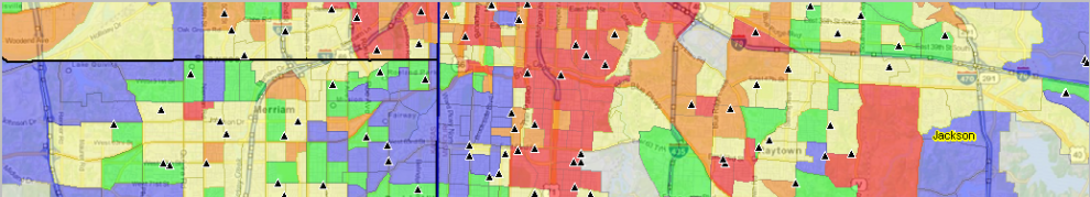
The following graphic illustrates the results of using the Shp2Shp tool to determine which block groups touch block group 48-85-030530-2 — a block group located within McKinney, TX. Shp2Shp determines which block groups touch this block group, then selects/depicts (crosshatch pattern) these block groups in the corresponding GIS map view.

Geographic Reference File
In the process, Shp2Shp creates a geographic relationship file as illustrated below. There are six block groups touching the specified block group. As shown in the above view, one of these block groups touches only at one point. The table below (derived from the XLS file output by Shp2Shp) shows six rows corresponding to the six touching block groups. The table contains two columns; column one corresponds to the field GEOID from Layer 1 (the output field as specified in edit box 1.2 in above graphic) and column 2 corresponds to the field GEOID from Layer 2 (the output field as specified in edit box 2.2 in above graphic). The Layer 1 column has a constant value because a query was set (geoid=’480850305302′) as shown in edit box 1.3. in the above graphic. Any field in the layer dataset could have been chosen. The GEOID may be used more often for subsequent steps using the GRF and further described below. It is coincidental that both layers/shapefiles have the field named “GEOID”.
| Layer 1 | Layer 2 |
| 480850305302 | 480850305272 |
| 480850305302 | 480850305281 |
| 480850305302 | 480850305301 |
| 480850305302 | 480850305311 |
| 480850305302 | 480850305271 |
| 480850305302 | 480850305312 |
Note that in the above example, only the geocodes are output for each geography/shape meeting the type of geospatial relationship. Any filed within either shapefile may be selected for output (e.g., name, demographic-economic field value, etc.)
How it Works — Shp2Shp Operations
The following graphic shows the settings used to develop the map view shown above.

See related section providing details on using the Shp2Shp tool.
Geographic Relationships Supported
The Select Relationships dropdown shown in the above graphic is used to determine what type of spatial relationship is to be used. Options include:
• Equality
• Disjoint
• Intersect
• Touch
• Overlap
• Cross
• Within
• Contains
See more about the DE-9IM topological model used by Shp2Shp.
Try it Yourself
See full details on how you can use any version, including the no fee versin, of CV XE GIS to use the Shp2Shp tools. Here are two examples what you can d. Use any of the geospatial relatoinships. Apply your own queries.
Using Touch Operation
Select the type of geographic operation as Touch. Click Find Matches button. The map view now shows as:

Using Contains Operation
Click RevertAll button. Select the type of geographic operation as Contains. Click Find Matches button. The map view now shows as:

Relating Census Block and School Attendance Zones
The graphic shown below illustrates census blocks intersecting with Joyner Elementary School attendance zone located in Guilford County Schools, NC (see district profile). The attendance zone is shown with bold blue boundary. Joyner ES SAZ intersecting blocks are shown with black boundaries and labeled with Census 2010 total population (item P0010001 as described in table below graphic). Joyner ES is shown with red marker in lower right.
– view developed using CV XE GIS and related GIS project; click graphic for larger view
See more about this application in this related Web section.
Join me in a Data Analytics Lab session to discuss more details about accessing and using wide-ranging demographic-economic data and data analytics. Learn more about using these data for areas and applications of interest.
About the Author
— Warren Glimpse is former senior Census Bureau statistician responsible for innovative data access and use operations. He is also the former associate director of the U.S. Office of Federal Statistical Policy and Standards for data access and use. He has more than 20 years of experience in the private sector developing data resources and tools for integration and analysis of geographic, demographic, economic and business data. Contact Warren. Join Warren on LinkedIn.